What bandwidth actually guarantees: the −3 dB point and the three-to-five-times rule
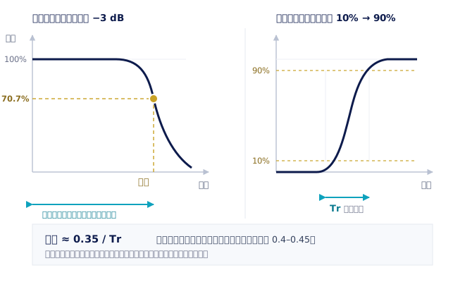
The 'bandwidth' on an oscilloscope's data sheet is not an on/off switch for whether you can see something; it is one marked point on an amplitude response curve. The manufacturer sweeps sine waves of constant amplitude across frequency and measures the amplitude the oscilloscope displays; when the displayed amplitude has fallen to −3 dB of the input (about 70.7%), that frequency is defined as the model's bandwidth. In other words, a 500 MHz oscilloscope is already displaying nearly 30% less signal at 500 MHz — it does not begin to have trouble after 500 MHz, and the attenuation in fact started quietly at much lower frequencies.
So bandwidth must not be matched to the signal frequency when selecting an instrument. The general rule of thumb is to take the oscilloscope bandwidth as three to five times the signal's highest significant frequency component. At three times, the amplitude error is roughly within a few percent, which is usable; at five times, the shape of the waveform — overshoot, ringing, the curvature of the edge — also stays trustworthy. If your job is to decide whether something is out of specification rather than merely whether a signal is present, lean towards five.
Conversely, buying too much bandwidth also has a price. The higher the bandwidth, the wider the noise bandwidth entering the front end, so the noise floor when measuring small signals gets worse; price and probe cost scale in proportion as well. Most R&S oscilloscopes (the R&S®MXO 3, R&S®MXO 4, R&S®MXO 5, R&S®RTM3000 and R&S®RTO6 families, for example) offer software-licensed bandwidth upgrades, and buying enough bandwidth for now and upgrading when the project genuinely moves up is more pragmatic than buying the top of the range in one go.
The real frequency content of a digital signal: look at the edge, not the clock
The mistake engineers make most often is picking bandwidth from the clock frequency — 'my bus runs at 100 MHz, so a 200 MHz oscilloscope should be more than enough'. In digital circuits that reasoning does not hold. A square wave is not a sine wave; it is the fundamental plus a series of odd harmonics, and it is those harmonics, far above the clock, that make the edge steep. The edges of a 100 MHz clock may carry energy extending above 1 GHz. What really determines how much bandwidth you need is the edge rate, that is, the rise time.
The relationship that converts rise time into frequency is extremely useful: for an oscilloscope with a roughly Gaussian response, bandwidth ≈ 0.35 / rise time, with rise time conventionally taken between the 10% and 90% points. For example, if you measure (or read from a component data sheet) an edge with a 1 ns rise time, the signal's highest significant frequency component is about 0.35 GHz, that is, 350 MHz; multiply by three to five and you need an oscilloscope of 1 GHz to 1.75 GHz — far beyond what 'a 100 MHz clock' intuitively suggests.
Note that the constant 0.35 is not universal. It comes from the assumption of a single-pole, Gaussian roll-off, which older analogue oscilloscopes and many low- to mid-bandwidth models do satisfy. But modern high-bandwidth oscilloscopes are usually designed with a flatter frequency response and a steeper roll-off — a 'near maximally flat' front end — in pursuit of measurement accuracy, and for those the constant falls somewhere between about 0.4 and 0.45. Which means that at the same bandwidth, an oscilloscope with a flatter response can actually measure a faster edge. In practice, use the system rise time the manufacturer's data sheet states rather than applying 0.35 everywhere. A flat frequency response across the whole band is one of the main design claims of the R&S®RTO6 family.
One more thing is easy to overlook: the rise time you measure is the combination of the signal's true rise time and the oscilloscope's own. The two add roughly as the root of the sum of squares, that is, 'measured² ≈ signal² + oscilloscope²'. When the oscilloscope's rise time approaches that of the signal, the edge you measure will be noticeably slower than it really is — which is the other reason to take three to five times the bandwidth.
Sample rate is not bandwidth: Nyquist is the lower bound, not the target
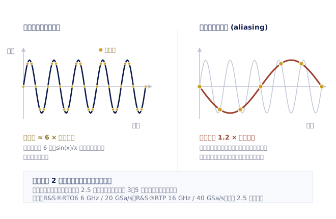
Sample rate (in GSa/s) and bandwidth are two independent specifications that are constantly conflated. Bandwidth describes how much frequency content the analogue front end lets in; sample rate describes how densely the ADC records it. What the front end blocks cannot be recovered by any sample rate; conversely, if what the front end lets in is undersampled, it appears on screen as a false signal — aliasing — which is more dangerous than not seeing it at all, because it looks real (see Fig. 1).
The Nyquist criterion says the sample rate must be greater than twice the highest frequency in the signal to avoid aliasing. That is a mathematical lower bound, not an engineering target. In practice an oscilloscope has to reconstruct a continuous waveform from discrete sample points using sin(x)/x interpolation, and at exactly twice the frequency the reconstruction quality is marginal at best; the general recommendation is a sample rate of at least 2.5 times the bandwidth, and most high-end models achieve three to five times. A few real numbers for comparison: the R&S®RTO6 family reaches 6 GHz of bandwidth with up to 20 GSa/s, and the R&S®RTP family 16 GHz with up to 40 GSa/s — both ratios above 2.5.
The trap that is easier to fall into is that the sample rate is often shared. On many oscilloscopes the ADC resources are interleaved between channels, so two channels run at full speed while all four channels leave each with half. On the R&S®MXO 5 family, for instance, the sample rate is up to 5 GSa/s with 2 channels and 2.5 GSa/s with 4, which is a typical interleaved architecture. By contrast the R&S®MXO 4 family specifies 5 GSa/s 'on all 4 channels simultaneously', and the R&S®MXO 3 family likewise offers 5 GSa/s — and in debugging scenarios that need several signals observed at once (gate drive, supply rail and bus together, say), 'sample rate available per channel simultaneously' is worth comparing far more than the maximum figure in the catalogue.
The check to run when selecting is simple: turn to the data sheet, find the sample rate on the row for the number of channels you intend to use at the same time, and compare it with the bandwidth. If the ratio falls below 2.5, the waveform detail you measure near the top of the bandwidth is already being discounted.
ADC bits: what separates 8-bit from 12-bit
This is the single largest differentiator among modern oscilloscopes, and also the one data sheets most easily pass over. The number of ADC bits (the vertical resolution) determines how many steps the full vertical range on screen is divided into. A traditional 8-bit ADC has only 256 steps; across the usual eight vertical divisions that is 32 steps per division. 10-bit is 1024 steps, four times 8-bit; 12-bit is 4096 steps, sixteen times 8-bit.
Why does this matter? Because real-world measurements are so often 'a small signal riding on a large one'. Typical situations: tens of millivolts of ripple to be seen on a 12 V supply rail; gate ringing to be seen on a 400 V switching node; small distortion to be found on a full-scale analogue signal. You have to set the vertical scale large enough to fit the large signal, and at that point the small signal is left with barely any steps at all — on 8-bit, tens of millivolts might fall inside one or two quantisation steps, so the waveform comes out as a coarse staircase, or is swamped by quantisation noise entirely. Move to 12-bit and the same setting leaves sixteen times as many usable steps, and the small signal finally grows a shape.
R&S's current models are clearly tiered on this point: the entry-level R&S®RTB 2 family and the general-purpose R&S®RTM3000 family use a 10-bit ADC, four times the vertical resolution of a traditional 8-bit model; the R&S®MXO 3, R&S®MXO 4 and R&S®MXO 5 families use a 12-bit ADC and maintain 12 bits at full sample rate, with no need to trade speed for resolution. The R&S®MXO 3 and R&S®MXO 5 families additionally have an HD high-resolution mode reaching up to 18 bits, while the HD mode of the R&S®RTO6 and R&S®RTP families reaches 16 bits.
Keep expectations of high-resolution (HD) mode correct: it works by low-pass filtering and averaging the sampled data, trading effective bandwidth for lower noise and more effective bits. It is excellent for measuring low-frequency supply ripple or analogue signals, but it will not turn an 8-bit instrument into a 12-bit one at full bandwidth. The native bit count is the hardware floor; HD mode is a bonus on top of it.
Memory depth: the tug of war between capture time and sample rate
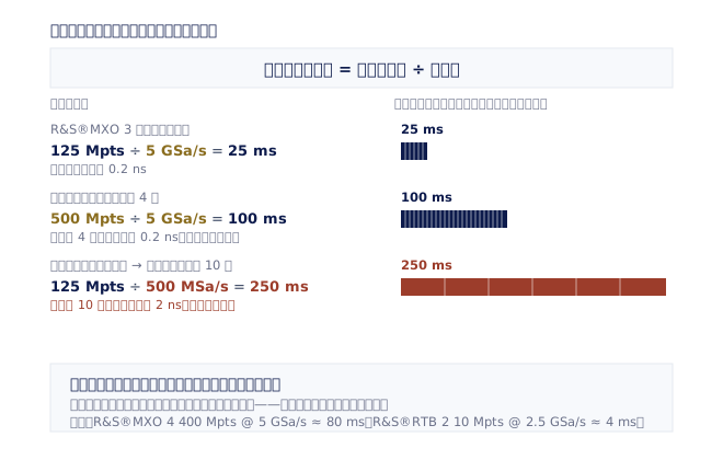
Memory depth (in Mpts or Msample) is the third specification that gets overlooked and yet decides how usable an instrument really is. The relationship between the three is one simple expression: continuous capture time = memory depth ÷ sample rate. Once the oscilloscope is triggered to acquire, sample points are pushed into memory until it is full.
That expression carries a brutal trade-off: as you stretch the timebase out to see a longer stretch of time, holding full sample rate consumes more memory, and when there is not enough memory the oscilloscope automatically reduces the sample rate. This is exactly the oddity so many people run into — the signal looks perfectly clear at a fast sweep, then you stretch the timebase to hunt for an anomaly that appears once every few seconds and the waveform detail turns to mush, because the sample rate has quietly dropped to a few MSa/s. The only way to keep a high sample rate across a long capture window is deep memory.
Real numbers make it vivid: the R&S®MXO 4 family ships with 400 Mpts per channel, which at its full 5 GSa/s allows about 80 milliseconds of continuous capture; the R&S®MXO 3 family ships with 125 Mpts per channel (about 25 milliseconds), upgradeable to 500 Mpts per channel (about 100 milliseconds); the R&S®MXO 5 family ships with 500 Mpoints per channel, upgradeable to 1 Gpoint. By contrast the entry-level R&S®RTB 2 family ships with 10 Msample, about 4 milliseconds at its maximum 2.5 GSa/s — enough for general debugging, but stretched thin if you need to capture tens of milliseconds of a boot sequence at full speed. The high-end R&S®RTO6 family ships with 200 Mpts expandable to 2 Gpts, and the R&S®RTP family reaches up to 3 Gpoints per channel, precisely for this kind of long, high-sample-rate requirement.
There is also one practical memory-saving feature: segmented memory. It records only a short stretch at each trigger event and skips the long blank intervals in between, so a limited memory can cover a very long observation period — ideal for bursty communications packets or intermittent faults. The R&S®RTM3000 family offers deep segmented memory upgradeable to 400 Msample, and the segmented memory of the R&S®RTB 2 family reaches 160 Msample.
The probe is part of the measurement, not an accessory
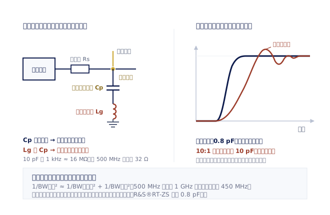
The last item, and the one most often treated as a giveaway: the probe. The idea to accept first is that what you measure is never what the circuit originally looked like, but what 'circuit plus probe' looks like. The instant the probe touches down, its input resistance, input capacitance and ground loop become part of the circuit under test — this is loading.
At low and medium frequencies, loading is dominated by the input resistance, and 1 MΩ usually has little effect. But as frequency rises, input capacitance takes over. The reason is that capacitive reactance falls inversely with frequency: 10 pF is about 16 MΩ at 1 kHz, effectively absent; at 500 MHz it is only about 32 Ω — the equivalent of hanging a few tens of ohms across your signal node. The result is that edges get slowed, ringing gets absorbed and timing gets shifted, and you receive no warning whatsoever. It is also why the ground spring of a passive probe matters far more than that long crocodile-clip ground lead: the inductance of a long ground lead resonates with the probe capacitance and manufactures ringing on fast edges that does not exist at all.
The second thing is that probe bandwidth caps the bandwidth of the whole system. System bandwidth is not the lower of the two but lower than either — combined roughly as the root of the sum of the inverse squares (1/BW_system² ≈ 1/BW_scope² + 1/BW_probe²). Put a 500 MHz passive probe on a 1 GHz oscilloscope and what you actually own is a measurement system of about 450 MHz, not 1 GHz. Buying a high-bandwidth oscilloscope and keeping the old probes means throwing the price difference away. The R&S® RT-ZP passive probe family covers 38 MHz to 700 MHz and is the choice for general debugging and cost-sensitive work; once the measurement frequency goes beyond that range, you have to move to an active probe.
An active probe has a built-in amplifier and can achieve both high input resistance and extremely low input capacitance at once, making it the solution with the least loading. The R&S®RT-ZS active single-ended probe family covers 1 GHz to 6 GHz with 1 MΩ input resistance and input capacitance as low as 0.8 pF (0.3 pF on the RT-ZS60) — set that against the ten-plus picofarads typical of an ordinary passive probe and it becomes clear why high-speed signals demand an active probe.
Next comes the judgement of which probe to use. If the signal is differential (USB, PCIe, automotive Ethernet, or the gate-source voltage of a switching supply), or if neither end of the signal is grounded, you need a differential probe: the R&S® RT-ZD active differential probe family covers 1 GHz to 4.5 GHz with under 1 pF of input capacitance, suited to high-speed digital differential pairs. If the target is a high-voltage floating node in power electronics (IGBT, SiC and GaN gate drive and drain voltage, or the three-phase voltages of an inverter), you need a high-voltage differential probe: the R&S®RT-ZHD high-voltage differential probe family measures up to 6000 V RMS and meets the CAT III 1000 V safety category. In environments with extremely high common-mode voltage and very strong noise, the R&S®RT-ZISO isolated probe system uses a power-over-fibre architecture to isolate the device under test from the oscilloscope completely, with a common-mode range of ±60 kV and still more than 90 dB of common-mode rejection ratio (CMRR) at 1 GHz.
As for current, an oscilloscope cannot measure it directly and needs a current probe to convert current into voltage. The R&S® RT-ZC current probe family uses a non-invasive clamp design covering 20 kHz to 120 MHz with current ranges up to ±2000 A, suited to current waveform analysis in switch-mode supplies, motor drives and electric vehicle systems. One easily overlooked specialist tool to add at the end: when measuring tiny ripple on a supply rail, a 1:1 power rail probe (the R&S® RT-ZPR power rail probe, 2 GHz / 4 GHz, with ±60 V of offset compensation) can shift the DC level away without attenuating the signal, leaving the oscilloscope's entire vertical range for those tens of millivolts of ripple — the same problem the ADC bit count addresses, solved from the other side, and in practice the two are normally used together.
A practical closing reminder: when making power measurements, the propagation delay of a voltage probe and a current probe are not the same, and a deskew calibration must be done first, or the instantaneous power you compute will be systematically wrong. R&S supplies deskew calibration fixtures such as the RT-ZF20, and this is a step not to be skipped before any power efficiency measurement.