
NF measures a ratio, not a power
Noise figure (NF) is often read as 'how much noise this component has'. It is not. NF measures how much this component has spoiled the signal-to-noise ratio. The definition starts from the noise factor (F): the signal-to-noise ratio at the input divided by the signal-to-noise ratio at the output, both measured with the source at the standard reference temperature of 290 K. Take the logarithm and NF = 10·log₁₀(F), in dB. F is always at least 1 and NF is always at least 0 dB.
Why a ratio? Because an amplifier that amplifies the signal by 20 dB also amplifies the noise that arrived at its input by 20 dB — the signal-to-noise ratio is not improved by amplification. The only thing that genuinely degrades it is the extra noise this stage adds by itself. So an ideal noiseless amplifier has F = 1 and NF = 0 dB whether its gain is 10 dB or 60 dB. That also resolves a common confusion: NF is independent of gain, and two front ends 30 dB apart in gain can have exactly the same NF.
For passive components there is a rule worth memorising first: a passive lossy component operating at ambient temperature — cable, connector, attenuator, filter, circulator — has an NF numerically equal to its insertion loss. A filter with 1.5 dB of loss has an NF of 1.5 dB. The rule matters because it turns the cost of 'that piece between the antenna and the LNA' into something calculable rather than a vague impression.
Finally, keep NF and noise floor apart: they are different things. NF is a relative quantity in dB and carries no bandwidth information; the noise floor is an absolute power in dBm and is tied to a bandwidth. Two receivers both with NF of 3 dB, one with a 200 kHz channel and one with a 100 MHz channel, have noise floors 27 dB apart. See dBm and ask about bandwidth; see dB and ask about the reference condition — the first reflex for reading any noise specification.
Where −174 dBm/Hz comes from: kTB and the 290 K convention
The thermal motion of electrons inside a resistor inevitably produces noise; this is a result of thermodynamics, not of poor design. The available noise power is N = kTB, where k is Boltzmann's constant, 1.38×10⁻²³ J/K, T is absolute temperature (K) and B is bandwidth (Hz). Put in T = 290 K and B = 1 Hz and the result is 4.00×10⁻²¹ W, which in dBm is −173.98 and is universally written as −174 dBm/Hz. Every RF sensitivity calculation starts from that number.
Why 290 K rather than a room temperature of 300 K? 290 K is the standard reference temperature T₀ laid down by the IEEE, equivalent to 16.85 °C — not the actual temperature of any laboratory, but a convention that lets NF specifications from around the world be compared, chosen because kT₀ happens to come out close to 4.00×10⁻²¹ W and therefore computes cleanly. If the laboratory works at 25 °C (298 K), the true noise temperature of the cold state is not 290 K; a deviation of this order, about 0.1 dB, is negligible when measuring a 3 dB mixer but has to be corrected when measuring a 0.5 dB LNA.
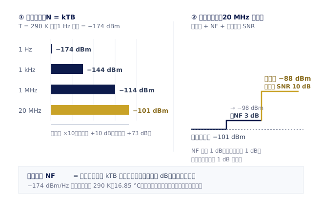
The bandwidth part is straightforward: noise floor = −174 dBm + 10·log₁₀(B). 1 kHz is −144 dBm, 1 MHz is −114 dBm, a 20 MHz LTE channel is −101 dBm and a 100 MHz 5G NR channel is −94 dBm. Add the receiver's NF for the actual noise floor, then add the signal-to-noise ratio demodulation requires and you have sensitivity: sensitivity = −174 + 10·log₁₀(B) + NF + required SNR. With a 20 MHz channel, NF of 3 dB and a required SNR of 10 dB, sensitivity is −88 dBm (Fig. 1). Set the required SNR to 0 dB and the −98 dBm that results is the minimum detectable signal (MDS).
Run the same expression backwards and a spectrum analyser's displayed average noise level (DANL) gives its equivalent noise figure: NF = DANL(dBm/Hz) + 174. If an analyser's DANL with the preamplifier on is −163 dBm/Hz, its equivalent NF is 11 dB. That conversion is useful when choosing measuring equipment: if the device under test has an NF of only 1 dB, measuring it directly with an analyser of 11 dB equivalent NF will be very hard work — you would need to add a low-noise amplifier stage in front, or switch to the vector-corrected cold-source method.
The Friis cascade: why the first stage decides the whole chain
A real receiver is a string of components: antenna → filter → LNA → mixer → IF amplifier → ADC. The noise factor of the whole chain is given by the Friis cascade formula: F = F₁ + (F₂−1)/G₁ + (F₃−1)/(G₁G₂) + …. The first thing to remember: every F and G in that expression is a linear ratio, not dB. Substituting decibels directly is the commonest calculation error on this subject, and the wrong answers it produces tend to look perfectly reasonable, which makes them hard to catch.
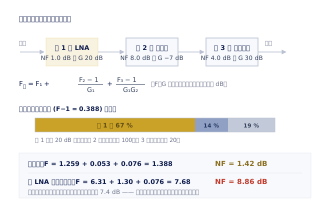
Take a set of real numbers (Fig. 2). First stage, an LNA: NF 1.0 dB (F₁ = 1.259), gain 20 dB (G₁ = 100). Second stage, a mixer: NF 8.0 dB (F₂ = 6.31), conversion loss 7 dB (G₂ = 0.20). Third stage, an IF amplifier: NF 4.0 dB (F₃ = 2.51), gain 30 dB. Substituting, F = 1.259 + 5.31/100 + 1.51/19.95 = 1.259 + 0.053 + 0.076 = 1.388, so the total NF is 1.42 dB. The whole chain is only 0.42 dB worse than that LNA on its own, and the second and third stages together contribute only 0.129 of the total excess noise of 0.388.
Now swap the order of those same three components — mixer first, LNA second: F = 6.31 + 0.259/0.20 + 1.51/19.95 = 7.68, a total NF of 8.86 dB. No part changed, no specification changed, and the order alone cost 7.4 dB. In a link budget 7.4 dB is roughly 5.5 times more transmit power, or more than halving the communication distance in free space. That is the quantified version of 'the first stage decides everything'.
The same reasoning explains why 'every decibel ahead of the LNA is expensive': the feeder, connectors, limiter and band-pass filter between the antenna and the LNA are all passive losses at ambient temperature, their NF equals their loss, they stand in the first position, their gain is less than 1, and they therefore amplify the noise of everything behind them back up again. 1 dB of feeder loss is very nearly 1 dB on the total NF — which is precisely why tower-mounted amplifiers and antenna-integrated LNAs exist. That said, more first-stage gain is not automatically better: pushing gain up drives the later stages towards compression and intermodulation distortion, the chain's third-order intercept (IP3) and its NF optimise in opposite directions, and the usable dynamic range is what the two of them leave in between. Front-end design is really the tuning of that balance, not the minimisation of NF on its own.
Noise temperature or noise figure: the territory of each convention
The same thing has a second notation: equivalent noise temperature (Te). Imagine the device under test as entirely noiseless, preceded by a resistor at temperature Te whose noise is exactly equal to the noise the device adds by itself. The conversion is Te = (F − 1)·T₀, with T₀ = 290 K. Side by side: NF 0.5 dB corresponds to Te 35 K, 1.0 dB to 75 K, 1.5 dB to 120 K, 2.0 dB to 170 K and 3.0 dB to 289 K.
Why two systems? Because the logarithmic dB scale flattens the differences in the low-NF region. 0.5 dB and 0.7 dB look only 0.2 dB apart; in noise temperature they are 35 K and 51 K — nearly half as much again. For satellite earth stations and radio astronomy that is a decisive difference: with the antenna pointed at cold sky, antenna noise temperature may be only 10 to 50 K, system noise temperature is Tsys = Tant + Te, and every degree of Te then shows up directly in the smallest signal that can be received. It is also why satellite links conventionally use G/T (antenna gain divided by system noise temperature, in dB/K) as their figure of merit rather than NF.
Conversely, the source in commercial wireless communications, EMC and general RF component testing is an antenna or a 50 Ω load at about room temperature in the first place, so the source noise is around 290 K, NF expresses it most intuitively, and it adds directly to the other dB terms in a link budget. So the convention can be remembered like this: use noise temperature where the source is cold and the NF very low; use noise figure where the source is at room temperature and dB terms are being summed. The two carry exactly the same information on different scales, and convert at any time.
One practical caution: a data sheet stating 'NF = 0.3 dB' converts to a Te of only 21 K, already close to the physical limit of GaAs and GaN low-noise devices at room temperature. When a markedly lower room-temperature NF is claimed, ask first whether it is NFmin measured at the optimum source reflection coefficient Γopt rather than the value actually obtainable in a 50 Ω system — both numbers can be true, but they are not answers to the same question.
How to measure it: the Y-factor, cold-source and gain methods
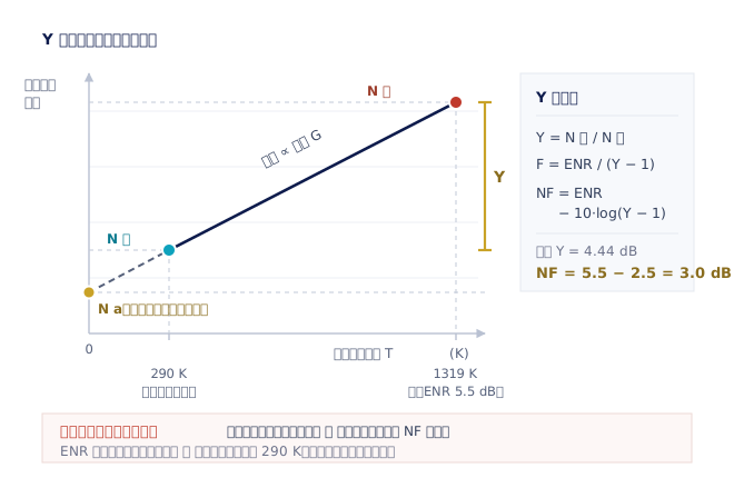
The most widespread method is the Y-factor method. An avalanche diode noise source puts out 'hot' noise with 28 V applied (equivalent temperature Th) and 'cold' noise with the power off (equivalent temperature roughly the ambient temperature Tc). The noise source is specified by its excess noise ratio (ENR) = 10·log₁₀((Th − Tc)/T₀), and the market divides broadly into low-ENR sources of 5 to 6 dB and high-ENR sources of around 15 dB. Measure the output noise power in the two states, Nh and Nc, take the ratio Y = Nh/Nc, and F = ENR(linear) / (Y − 1), or in dB, NF = ENR(dB) − 10·log₁₀(Y − 1). With a 5.5 dB ENR noise source and a measured Y of 4.44 dB, NF = 5.5 − 2.5 = 3.0 dB (Fig. 3).
The picture behind the Y-factor method is a straight line: output noise power plotted against source noise temperature is linear, its slope is proportional to gain, and extrapolating the line back to absolute zero gives an intercept equal to the noise the device adds by itself. The cold and hot measurement points exist only to establish that line. The picture also shows its weakness directly: the smaller the power difference between the two points (that is, Y), the greater the uncertainty in the slope. The higher the device's NF, the smaller Y and the less accurate the measurement — so a high-NF device suits a high-ENR noise source, while a low-NF device is better served by a low-ENR source, because a low-ENR source changes impedance less between its on and off states and therefore brings less mismatch error with it.
The cold-source method uses only the 'cold' state: terminate the device's input with a room-temperature 50 Ω load, measure its output noise power, obtain the gain separately, and the noise the device adds can be calculated. It asks for more than the Y-factor method — an accurate gain value is required, and the measuring receiver's own noise contribution has to be subtracted first — but it repays the effort: gain is obtained from S-parameters, so a vector network analyser's full error correction can take source and load mismatch into account. This is exactly the route taken by the noise figure options of modern vector network analysers (the R&S®ZNA and R&S®ZNB) and signal analysers (the R&S®FSW and R&S®FSV3000): no noise source, no ENR uncertainty, and markedly better accuracy than the Y-factor method when measuring an LNA below 1 dB. The price is a more complex setup, and a measuring receiver that has to be quiet enough.
The third is the gain method (also called the direct method or noise floor method): terminate the input with a 50 Ω load, measure the device's output noise power density directly with a spectrum analyser, and subtract the gain and −174 dBm/Hz to get NF. The advantage is that it needs no extra hardware — an analyser and a load will do; the disadvantage is that it only holds when the device's gain plus NF is enough to lift the noise clear of the analyser's own noise floor. As a rule of thumb, the device needs more than 30 dB of gain, or an NF above 10 dB in its own right (measuring a complete receiver or a downconverter module, say), for the method to mean anything. Point it at an LNA with 1 dB NF and 15 dB gain and what you measure is the analyser's data sheet.
Why the numbers disagree: four error sources, and how to compare data sheets
Mismatch is what costs you most easily. Noise figure is defined for a particular source impedance: a transistor's noise behaviour is described completely by four noise parameters — the minimum noise figure NFmin, the optimum source reflection coefficient Γopt (magnitude and phase) and the equivalent noise resistance Rn. NFmin is only obtained when the source impedance is exactly Γopt, and Γopt is almost never 50 Ω, nor the power-matched point. So the NFmin on a component data sheet and the value you measure in a 50 Ω fixture were never going to be the same; neither is wrong, the conditions differ. Obtaining all four noise parameters means sweeping several source impedances with an impedance tuner, which is work of another order.
The second is the measuring receiver's own noise figure. Every method measures the cascade of 'device under test + measuring receiver', and the second stage has to be backed out with Friis — a step called second-stage correction, which presupposes that the measuring receiver's NF has itself been accurately calibrated. The smaller the device's gain, the more the second stage weighs: measuring an LNA with 20 dB of gain it is almost negligible, while measuring a mixer with 7 dB of conversion loss it may contribute most of the reading. In that situation the right approach is to put a low-noise preamplifier of known characteristics in front of the measuring receiver.
The third is the noise source itself. ENR is a calibration table that varies with frequency, not a single number, and it drifts over time; calibration once a year is the usual recommendation. An uncertainty of 0.2 dB on ENR essentially passes through untouched as 0.2 dB of uncertainty on NF. Adapter and cable losses between the noise source and the device have to be subtracted separately, and those losses themselves contribute noise at ambient temperature. The fourth is temperature: the Y-factor method assumes the cold state is at 290 K, but a laboratory is usually at 23 to 27 °C (296 to 300 K), and the diode also self-heats after the noise source has been powered for a long time. Modern noise figure measurement software all provides an ambient temperature field for the correction — fill it in.
Two further things are common in practice but never printed on a data sheet. One is external interference: noise figure measures extremely weak noise powers, and the laboratory's Wi-Fi, a mobile base station, even the switching noise of LED lighting can land in the passband — particularly noticeable when measuring components near 2.4 GHz, and sometimes a shielded room is needed. The other is insufficient averaging: a noise measurement is statistical by nature, the standard deviation of the reading is inversely proportional to √(B·τ), and rushing to finish yields a number that looks attractive and cannot be reproduced. Finally, comparing two data sheets means aligning at least five things: the measurement frequency, whether the source impedance was 50 Ω or Γopt, whether the value is typical or guaranteed, whether fixture and cable losses are included, and the ambient temperature and whether second-stage correction was applied. With those five aligned, comparing NF becomes a question with an answer.