
What jitter is: the time error of an edge, and also phase noise
Jitter is defined as the deviation of a signal's significant instants — usually the moment an edge crosses the decision threshold — from their ideal positions in time. The unit can be the second (ps or fs for high-speed signals) or the unit interval (UI), where 1 UI is the length of one bit, the reciprocal of the data rate. At 10 Gbit/s, 1 UI = 100 ps, so '0.3 UI of jitter' is 30 ps. Expressing jitter in UI makes it comparable across data rates; expressing it in seconds makes it directly addable to clock specifications, and both forms appear on data sheets.
Telecommunications gives the slow part its own name: phase variation above 10 Hz is called jitter and below 10 Hz is called wander. The boundary is not physical but practical — a receiver's clock recovery loop can follow the slow part and cannot follow the fast part, and the consequences differ, so the standards manage them separately.
More importantly, jitter and phase noise are two coordinate systems for the same thing. Write a clock as x(t) = A·sin(2π·f₀·t + φ(t)); the phase disturbance φ(t) converts into a time disturbance as Δt = φ / (2π·f₀). So integrating the single-sideband phase noise L(f) across the band of interest gives the RMS phase error φrms = √(2·∫L(f)df) in radians, and dividing by 2π·f₀ gives the RMS time jitter. A concrete example: on a 100 MHz clock, φrms computed over the specified integration band comes to 63 µrad, which converts to 63×10⁻⁶ ÷ (2π×10⁸) ≈ 100 fs of RMS jitter.
That conversion carries a condition that has to travel with it: the integration band. Different standards specify different upper and lower limits (12 kHz to 20 MHz is common in optical communications), and a different band gives a different jitter number — just as phase noise is not a specification without an offset frequency, a point covered in full in Phase Noise: What It Is, What It Costs, and How It Is Measured. The practical division of labour is this: the frequency domain (a phase noise analyzer) suits a clean periodic clock and identifying noise sources by frequency; the time domain (an oscilloscope) suits a serial signal carrying data and decomposing the jitter into its components.
TIE: the starting point, and the hidden variable of the reference clock
Almost all serial-signal jitter analysis starts from the time interval error (TIE): take every edge instant you measured, subtract the instant at which it should have occurred, and you have a TIE sequence. TIE is an accumulating quantity — if the actual frequency is slightly higher than the ideal frequency, TIE walks away monotonically with time. Taking an FFT of the TIE sequence gives the jitter spectrum, in which periodic jitter shows up as discrete lines, and that is usually the fastest route to a noise source: a line at 33 kHz sends you to look at the switch-mode supply, a line at the same frequency as a nearby clock sends you to look at crosstalk.
The crux is who decides 'the instant at which it should have occurred', and there are two common choices whose answers can differ several-fold. The first is a constant-frequency reference: a least-squares fit across the whole record produces an ideal clock of fixed frequency. This counts all the low-frequency wander into TIE, gives the largest number, and suits examining the long-term behaviour of the clock itself. The second is a clock recovery (CDR) reference: a phase-locked loop conforming to the standard's own definition, with a specified order and loop bandwidth (many serial standards specify the data rate divided by 1667), extracts the clock from the data stream. Because a real receiver works exactly this way — it follows slow jitter — this method is equivalent to high-pass filtering the TIE and leaves only the part the receiver cannot follow.
This regularly starts arguments on the bench: on the same waveform, engineer A measures 12 ps RMS with a constant-frequency reference and engineer B measures 2.5 ps RMS with the standard's CDR, and neither of them has made an error. So any jitter figure has to be reported together with the reference clock setting; if the specification cites an interface standard, then the loop bandwidth and order that standard prescribes are the ones to set. Modern oscilloscopes implement CDR in software, which has the advantage that one captured record can be re-analysed repeatedly with different CDR settings, without measuring again.
Beyond TIE there are two other common measures that mean different things. Period jitter is the deviation of each clock period's length from the ideal period; cycle-to-cycle jitter is the difference in length between two adjacent periods. Both are local quantities, neither accumulates, and their numbers are usually far smaller than TIE. The setup and hold margins that digital designers care about are mostly read off period jitter, while the eye closure that a serial link cares about must be read off TIE. Putting a period jitter number into a field asking for TIE will badly understate the problem.
RJ is unbounded, DJ is bounded, and why they cannot be added
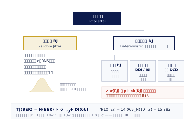
The first cut in decomposing jitter divides total jitter (TJ) into random jitter (RJ) and deterministic jitter (DJ) (Fig. 2). RJ comes from thermal noise, shot noise and 1/f noise, follows a Gaussian distribution and has no upper bound in theory — the longer you measure, the larger the peak-to-peak value you see. RJ can therefore only be expressed as an RMS value σ; any specification marked 'RJ peak-to-peak = x ps' without stating a sample count or a BER is self-contradictory on its face.
DJ, by contrast, is bounded, can reasonably be described peak-to-peak, and can be broken down further. Periodic jitter (PJ) comes from switch-mode supply ripple, reference spurs in a phase-locked loop and crosstalk from nearby clocks; it shows up as discrete lines in the TIE spectrum, and identifying the frequency usually identifies the culprit. Data-dependent jitter (DDJ), also known as inter-symbol interference (ISI), arises because the channel has frequency-dependent loss and reflections, so the residue of the preceding few bits shifts the position of this edge; it is tied to the bit pattern, it is repeatable, and the remedies are equalisation and pre-emphasis. Duty cycle distortion (DCD) comes from rising and falling edges having different delays, or from the decision threshold sitting off the centre of the signal, and appears on an eye diagram as the crossing point moving up or down, or as the crossing-point histogram splitting into two clumps. There is also a class of bounded jitter uncorrelated with the data (BUJ), typically originating in crosstalk from an adjacent channel.
Why can RJ and DJ not simply be added? Because the two numbers are not the same kind of quantity. σ is the dispersion parameter of an unbounded distribution, and a peak-to-peak value is the full span of a bounded one — adding them is as undefined as adding a standard deviation to a maximum. Even within a class the addition rules differ: mutually independent RJ components add in RMS (σtotal = √(σ₁² + σ₂²)), whereas DJ components add linearly only in the worst case and should strictly be convolved. To obtain a usable total jitter you must first specify a BER, which is exactly why the dual-Dirac model in the next section exists.
How does an instrument separate them? There are three main routes. One is tail fit, extrapolating σ and DJ from the Gaussian tails on either side of the histogram. Two is the spectral method, taking an FFT of the TIE and assigning the discrete lines to PJ and the flat noise floor to RJ. Three is pattern analysis, averaging each bit position over a known repeating pattern, so that the variation of the means is DDJ and the residual is the random component. Different methods have different strengths in different situations, which is also why the split between RJ and DJ for the same data can come out differently under different software or different settings — when comparing two reports, first confirm that the same decomposition algorithm and the same pattern length were used.
Dual-Dirac and the bathtub curve: where a total jitter at 10⁻¹² comes from
The industry's standard compromise is the dual-Dirac model: DJ is simplified into two Dirac impulses separated by DJ(δδ), and each impulse is convolved with a Gaussian of standard deviation σ. The value of the model is not how accurately it describes reality but that it turns total jitter into a straight line you can extrapolate along: TJ(BER) = N(BER) × σRJ + DJ(δδ). N(BER) is a coefficient read from a table: 9.507 at a BER of 10⁻⁶, 11.996 at 10⁻⁹, 12.723 at 10⁻¹⁰, 14.069 at 10⁻¹², and 15.883 at 10⁻¹⁵. For the same device under test, moving the BER condition from 10⁻¹² to 10⁻¹⁵ adds about 1.8 σ to the total jitter.
One easily misunderstood point is worth settling first: the DJ(δδ) obtained from a dual-Dirac fit is not the real peak-to-peak DJ. It is a model parameter and is usually smaller than the true value. Writing DJ(δδ) into a report as 'maximum deterministic jitter' is the most common way this model is misused, and one of the common reasons two reports fail to agree.
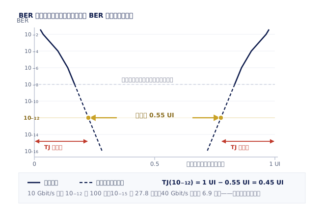
Plotting the result as a bathtub curve is the most intuitive presentation (Fig. 3): the horizontal axis is the position of the sampling point within the unit interval, and the vertical axis is the bit error ratio (BER) on a logarithmic scale. With the sampling point near the crossing the error ratio approaches 0.5, and as it moves towards the centre of the eye the ratio falls steeply, forming a sheer wall on each side. In the linear region of each wall (a straight line on the logarithmic vertical axis) the slope is set by σRJ and the horizontal position by DJ, which is what makes extrapolation possible. Take the horizontal line at BER = 10⁻¹² and its intersections with the two walls: the distance between them is the eye opening at that BER, and 1 UI minus it is TJ(10⁻¹²).
Why extrapolate rather than measure directly? Time. Actually observing an error ratio of 10⁻¹² at 10 Gbit/s means sending at least 10¹² bits, about 100 seconds, and having statistical confidence in it means several times that again; measuring 10⁻¹⁵ at the same 10 Gbit/s needs 10¹⁵ bits, about 27.8 hours, and even raising the rate to 40 Gbit/s still takes 6.9 hours. The premise of extrapolation is that the tails really are Gaussian; if the system conceals a mechanism of low probability but large amplitude — occasional crosstalk, a supply surge, a thermal event — the real bathtub curve will depart from the straight line at low BER, and the TJ an oscilloscope extrapolates will then be optimistic compared with what a bit error ratio tester (BERT) measures. On a design with only a sliver of margin left, sweeping a real bathtub curve with a BERT is not the place to economise.
How to read an eye diagram: eye width, eye height and what causes each
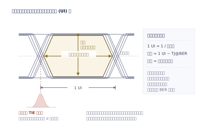
An eye diagram takes the many thousands of unit intervals you measured, aligns them to the recovered clock and overlays them on one plot (Fig. 1). The diamond-shaped region that opens in the middle is the eye: the horizontal opening is the eye width, representing how far the receiver's sampling instant may shift and still decide correctly; the vertical opening is the eye height, representing how much amplitude margin is left for the decision. The relationship between eye width and total jitter is direct: eye width ≈ 1 UI − TJ(BER), so an eye width figure is also meaningless without a stated BER.
Horizontal closure and vertical closure have different causes and must be looked at separately. Eye width is eaten mainly by jitter; eye height is eaten mainly by amplitude noise, channel insertion loss and inter-symbol interference. Mistaking vertical closure caused by channel loss for a clock quality problem is a very common debugging detour. The position of the crossing point speaks as well: a crossing that does not sit at the centre of the amplitude (at 45% or 55%, say) points to duty cycle distortion, and a crossing-point histogram that splits into two clumps rather than a single Gaussian usually indicates significant DCD or PJ.
An eye diagram is a statistical result, not a snapshot. The longer you measure and the more bits you overlay, the further the tails of the random jitter reach and the more closed the eye looks — so 'the eye is open' is not a conclusion unless it comes with a BER or a sample count. The standard practice is a mask test to the relevant specification, or reading the contour of the eye at a specified BER directly. Most modern oscilloscopes no longer overlay traces with a hardware trigger: they capture a long waveform first, then rebuild the clock with software CDR and accumulate the statistics. The advantage is that the same record can be re-analysed with different CDR settings and different equaliser settings as often as you like, reducing the cost of 'try another assumption and look again' to zero.
One precondition has to be met first: an eye diagram cannot be better than the front end. Insufficient oscilloscope bandwidth slows the edges and closes the eye spuriously in both the horizontal and the vertical direction, so what you measure is the instrument's low-pass response rather than the device under test; probe loading likewise changes the very edge you are trying to measure. Those trade-offs — the relationship between bandwidth and rise time, how high the sample rate should be, how to choose a probe — are discussed in full in Oscilloscope Bandwidth, Sample Rate and Probes, and it is worth confirming those front-end conditions hold before any jitter measurement.
How good the instrument has to be: bandwidth, sample rate and the scope's own jitter floor
The bandwidth requirement starts from the edge. The fundamental (Nyquist) frequency of an NRZ signal is half the data rate, so 5 GHz at 10 Gbit/s; but jitter measurement looks at the instant the edge crosses the decision threshold and must preserve the shape of that edge, which in practice means including at least the third harmonic (15 GHz), and up to the fifth (25 GHz) for fine edge analysis. The consequence of insufficient bandwidth is not merely 'slightly blunter edges' — the measured TIE acquires a systematic bias, whose direction depends on how the front-end noise converts into time error through the edge slope.
The sample rate must be high enough for the interpolation algorithm to reconstruct the threshold crossing reliably. The rule of thumb is a sample rate of at least 4 times the bandwidth, with sin(x)/x interpolation; when the sample rate is too low, the exact position of the edge between two sample points can only be guessed at, and the interpolation error turns directly into spurious jitter. Memory depth matters just as much: RJ/DJ decomposition must cover enough repetitions of the pattern, and too short a capture leaves DDJ poorly estimated and the tails of the RJ never sampled at all.
The item most easily overlooked is the oscilloscope's own jitter floor — the jitter of its sampling clock, usually specified in fs RMS. It adds to the device under test in RMS: σmeasured = √(σDUT² + σinstrument²). That expression tells you directly how good an instrument you need: if the instrument floor equals the device under test, the measured value comes out 41% high; if the floor is half the device under test, 12% high; if a third, only 5.4% high. So the rule of thumb that 'the instrument's jitter floor should be below a third of the device under test' is not an arbitrary saying — it is exactly what this expression gives. Most vendors' software allows a known instrument floor to be subtracted in RMS, but subtraction can only correct a systematic bias; it cannot recover resolution that has been swamped.
Vertical noise can also masquerade as jitter: as the edge crosses the decision threshold, a voltage noise of Δv becomes a time error of Δt = Δv ÷ (dv/dt) through the edge slope. The slower the edge, the more jitter the same vertical noise converts into — which is why an oscilloscope with a low-noise front end measures less jitter on a slow-edged signal, and why that smaller number is the correct one. Finally, instrument type: a real-time oscilloscope (the R&S®RTP, R&S®RTO6 and R&S®MXO 5, for example) can capture single-shot and supports re-analysis with software CDR and equalisers, and is the mainstay for debugging and jitter decomposition; a sampling oscilloscope has higher bandwidth and a lower intrinsic jitter floor but needs a repetitive signal and an external clock; a bit error ratio tester (BERT) gives you a real BER but no waveform. The three are complementary and do not replace one another. The probe is equally part of the measurement chain: signals on a board need a low-loading active differential probe (the R&S®RT-ZD series, for example) or a modular probe system (such as the R&S®RT-ZM), or the probe itself will change the very edge you are trying to measure.