
What phase noise is: the skirt beside the carrier
An ideal oscillator puts out a perfect sine wave, which on a spectrum would be a single line of infinitesimal width. A real oscillator does not. Write its output down mathematically and it becomes a sine wave with a little random fluctuation added to the amplitude and a little random fluctuation added to the phase: the amplitude term is AM noise, the phase term is phase noise. Because frequency is the rate of change of phase with time, a phase that jitters means an instantaneous frequency that jitters too — so what phase noise physically describes is short-term frequency instability.
Feed that signal into a spectrum analyser and the line that should have been a line becomes a mountain: the carrier in the middle, and on either side a continuous noise skirt falling away as it extends outward. That skirt is what phase noise looks like in the frequency domain. It is not a spur: spurious signals are discrete, needle-thin single lines, usually traceable to supply ripple, reference leakage or the comparison frequency of a phase-locked loop, and because their cause and their cure are different from phase noise, data sheets normally specify them separately.
Note that phase noise is a short-term quantity. An oscillator drifting with temperature, or ageing by a few ppm a year, belongs to long-term stability and frequency accuracy, which are measured with entirely different figures of merit. The same physics described in the time domain is Allan variance / Allan deviation, and described in the frequency domain it is phase noise; the two convert into each other, they simply suit different observation timescales — stability from seconds to hours is habitually read as Allan deviation, jitter below a millisecond as a phase noise curve. The R&S®FSWP phase noise analyser offers both presentations, and can compute Allan variance directly from the phase noise data.
Why dBc/Hz? The offset frequency is the other half of the specification
The quantity the industry uses is single-sideband phase noise L(f), defined roughly as the single-sideband noise power measured in a 1 Hz bandwidth at an offset f from the carrier, divided by the total carrier power. Take the logarithm and the unit is dBc/Hz — the 'dBc' says relative to carrier, the '/Hz' says already normalised to a 1 Hz bandwidth.
Neither normalisation is cosmetic. Dividing by carrier power makes the specification independent of how much you amplify or attenuate the signal: change the source's absolute output level and carrier and skirt move together, so the ratio does not move. Normalising to 1 Hz makes the specification independent of the resolution bandwidth (RBW) used for the measurement: noise power measured in a 100 Hz RBW is about 20 dB higher than in a 1 Hz RBW, and without the normalisation every change of setting would produce a different number and no two reports could be compared.
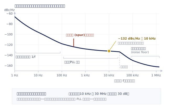
But the half that actually goes missing is the other one: the offset frequency, meaning how far from the carrier. Phase noise is fundamentally a curve, not a number (see Fig. 1). It is usually worst close in, falls away in segments as you move out, and finally flattens at large offsets into a broadband noise floor that has nothing to do with the carrier. How large is the difference? Take a real example: on the R&S®SMA100B RF and microwave signal generator, single-sideband phase noise at a 10 GHz carrier and 10 kHz offset is typically −132 dBc/Hz, while at the same 10 GHz carrier the measured wideband noise at 30 MHz offset is −162 dBc/Hz. Same instrument, same carrier, and the offset point alone accounts for a full 30 dB. So when someone says 'this one's phase noise is −132' without naming an offset, the sentence has conveyed nothing you can use.
The carrier frequency is part of the conditions too. For a source synthesised by multiplication or by a phase-locked loop, multiplying the frequency by N degrades phase noise in theory by 20·log₁₀(N) dB — the higher the frequency, the harder it is to keep clean. Data sheets therefore state the figure per carrier: the internal phase noise of the R&S®FSW signal and spectrum analyser, for instance, is typically −136 dBc/Hz at a 1 GHz carrier and 10 kHz offset, and −133 dBc/Hz at a 10 GHz carrier at the same 10 kHz offset.
What it actually costs you
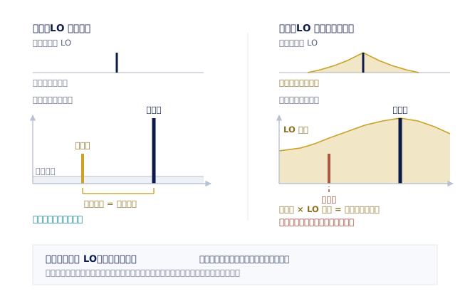
The first cost turns up in receivers, and it is called reciprocal mixing. What a mixer does is multiply the input signal by the local oscillator (LO). If the LO were a clean line, only the channel you want would be translated to the IF. But the LO carries a skirt, so an adjacent-channel interferer tens of dB stronger than your wanted signal multiplies with that skirt and smears a blanket of noise into your IF passband, raising the effective noise floor of that channel directly. The consequence: the receiver's dynamic range is limited not by noise figure but by the spectral purity of the local oscillator. The offset that matters here is simply how far away the interferer sits — whatever the channel spacing is, that is the offset to read. It is also why spectrum analysers put their own phase noise in the headline specifications: an analyser measuring a small signal runs into exactly the same physical limit.
The second cost turns up in modulated systems, as degraded EVM (error vector magnitude). Every symbol on a constellation diagram carries information in its phase; if the carrier phase jitters, the symbol point wanders in a circle on the constellation, and when it wanders across a decision boundary that is an error. Integrating the phase noise curve over the offset range you care about gives an RMS phase error in radians, and that radian value is approximately the EVM floor imposed by phase noise. Which explains why phase noise nobody worried about in the QPSK era becomes a project killer at 256QAM and 1024QAM: the denser the constellation, the smaller the phase wander it tolerates. In OFDM systems there is a further split: the part of the curve below the subcarrier spacing produces a phase rotation common to all subcarriers (common phase error) and can be tracked out with pilots; the part above the subcarrier spacing becomes inter-carrier interference (ICI), which no equaliser can remove and which is therefore a hard floor. To verify any of this, the test source itself has to be cleaner than the device under test — the R&S®SMBV100B vector signal generator, for example, achieves 0.2% EVM on a 20 MHz LTE signal precisely so that the EVM you measure reflects the device and not the generator.
The third cost turns up in clocks and digital systems, where the name changes to jitter. Phase deviation divided by angular frequency is time deviation, so after integrating phase noise over the offset band of interest to obtain an RMS phase error, dividing by 2π·f₀ converts it into RMS time jitter in seconds. This is especially lethal for high-speed ADCs and DACs: sampling clock aperture jitter limits SNR directly, and the higher the input signal frequency the more visible it becomes — the same clock that copes measuring a 100 MHz signal runs out of room at 3 GHz. SerDes jitter budgets and radar phase coherence come back to the same curve. Note that the integration band is part of the specification: different standards prescribe different limits, and a different integration band gives a different jitter number.
Measuring it (1): the direct spectrum analyser method and its ceiling
The most direct approach is to feed the signal under test into a spectrum analyser, measure the power of the skirt beside the carrier, and let the instrument normalise back to a 1 Hz bandwidth and subtract the carrier power. Most modern signal and spectrum analysers have a built-in phase noise measurement that handles RBW normalisation, detector correction and the stitching together of several sweep segments, so the operation is not difficult.
The method has three built-in limits, though. First, and hardest: the analyser's own local oscillator has phase noise too, so what you see is whichever of the two — device under test or analyser — is worse. When the device is cleaner than the analyser, all you have measured is the analyser's data sheet, and the result says nothing about the device. Second, the direct method sees total power and cannot separate amplitude noise from phase noise; where the device's AM noise is not negligible the result is pessimistic. Third, very close to the carrier (offsets of a few hertz to a few tens of hertz) it needs an extremely narrow RBW, sweep time grows, and the device's own frequency drift during that time smears the skirt wider.
So the direct method's place is clear: where the device under test is clearly worse than the analyser (in practice one likes at least 10 dB of margin) it is a fast, convenient, always-available check, well suited to a production go/no-go decision or to early development screening. Where the ceiling lies depends on the instrument — the flagship R&S®FSW signal and spectrum analyser, for instance, has an internal phase noise typically −136 dBc/Hz at a 1 GHz carrier and 10 kHz offset, and that same number marks the limit of what you can credibly measure with it by the direct method.
Measuring it (2): the phase detector method, and why cross-correlation pushes the floor down
A dedicated phase noise analyser takes a different route. A reference source is first phase-locked to the device under test in quadrature (90 degrees apart), and the two are fed to a phase detector. At the quadrature point the detector's output voltage is proportional to the phase difference between them, and the carrier itself has been cancelled. Once the carrier is gone, the following stages can apply high gain and do FFT analysis at baseband, with far more dynamic range available than 'finding small noise next to a large carrier' ever allows. The method has a useful side effect as well: it is inherently sensitive to phase and insensitive to amplitude, so it separates phase noise from amplitude noise.
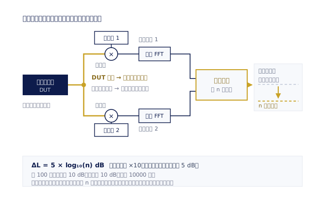
But the problem has only been deferred by one step: you need a reference source cleaner than the device under test, and the better the device, the less realistic that requirement becomes. Cross-correlation exists to get around it. The signal under test is fed simultaneously into two entirely independent measurement channels, each with its own reference source and phase detector, both looking at the same device at the same time. The key point is this: the device's phase noise is one and the same signal to both channels, so it is correlated; each channel's own reference noise, detector noise and amplifier noise are independent of the other's, so they are uncorrelated. Average the cross spectrum of the two channels and the correlated part survives while the uncorrelated part is pushed down as the number of averages rises — so the effective noise floor can fall below the noise of a single channel.
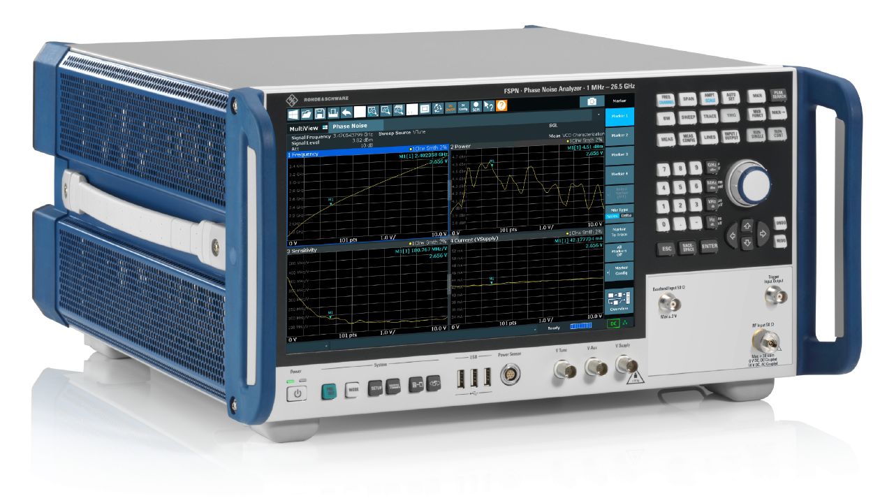
The price is time, and it grows on very unfriendly terms. The improvement follows ΔL = 5 × log(n) dB, where n is the number of correlations: 100 correlations buy 10 dB, and another 10 dB costs 10,000. This is exactly why dedicated instruments make the number of correlations a user-adjustable parameter, and why, when comparing two phase noise reports, you must always ask how many correlations were used and how long the measurement took. The R&S®FSPN phase noise analyser and VCO tester adopts this trade-off explicitly: two internal low-phase-noise synthesisers and a real-time cross-correlation engine, so production can trade few correlations for speed while development trades more correlations for depth, with a typical phase noise floor of < −163 dBc/Hz (1 GHz carrier, 10 kHz offset, 1 Hz RBW). The R&S®FSWP phase noise analyser and VCO tester in the same family reaches < −166 dBc/Hz (1 GHz, 10 kHz offset), covers 1 MHz to 8 / 26.5 / 50 GHz and extends to 325 GHz with external mixers; both measure phase noise and amplitude noise simultaneously, and both offer a residual (additive) phase noise mode for the noise a component itself adds.
Incidentally, instruments of this class usually handle VCO (voltage-controlled oscillator) characterisation as well — a built-in low-noise DC supply sweeps the tuning voltage automatically and captures frequency, sensitivity, output power and current consumption against voltage in one pass. The reason is straightforward: the VCO is where phase noise problems most often originate, and its phase noise correlates strongly with tuning voltage, load and supply noise, so measuring the two separately loses the point.
How to read the plot, and how to compare two data sheets honestly
On a standard phase noise plot the horizontal axis is offset frequency (logarithmic, commonly from 1 Hz or 10 Hz out past 10 MHz) and the vertical axis is L(f) in dBc/Hz, all negative, lower being better. The curve generally runs from upper left to lower right in segments: steepest closest to the carrier (flicker noise dominates), then a gentler slope through the middle, and finally flat at large offsets — the broadband noise floor. The break points themselves tell a story: the loop bandwidth of a phase-locked loop often leaves a distinct shoulder or bump on the curve, because inside the loop bandwidth the loop has carried the reference source's noise up with it, while outside the loop bandwidth what you see is the voltage-controlled oscillator's own noise. The thin spikes on the curve are not phase noise, they are spurs, and specified values normally exclude them explicitly.
Then comes the part that costs people most in practice: comparing two data sheets. At least six things have to be aligned. One, is the carrier frequency the same — a figure at 1 GHz cannot be set against a figure at 10 GHz. Two, is the offset frequency the same, which is the commonest trap of all: the R&S®SMA100B states its single-sideband phase noise at a 10 GHz carrier and 10 kHz offset, while the R&S®SMB100B RF signal generator states its spectral purity at a 10 GHz carrier and 20 kHz offset, and because the conditions differ the numbers cannot simply be subtracted. Three, is it typical (typ.) or specified (spec.) — a typical figure is usually several dB better and does not form part of factory acceptance. Four, does the quoted model include the relevant options: low phase noise in a signal generator often comes from options, and the R&S®SMA100B for instance offers R&S®SMAB-B709 low phase noise, R&S®SMAB-B710 improved close-in phase noise and R&S®SMAB-B711 ultra-low phase noise, so a base unit and a fully optioned unit are not the same instrument. Five, which reference oscillator is fitted — whether an OCXO option is installed changes the close-to-carrier part of the curve directly. Six, the measurement conditions themselves: how many cross-correlations, how long the measurement ran, and whether the number includes amplitude noise.
One last piece of advice is about order of operations: do not read the data sheet and then decide which offset you care about; decide from the application which offset you care about and then go back to the data sheet. A receiver looks at the offset corresponding to the channel spacing; an OFDM system looks at the two segments either side of the subcarrier spacing; an ADC clock looks at the jitter integration band; a PLL design looks inside and outside the loop bandwidth. Pin the offset down and comparing two data sheets becomes a question with an answer, rather than a contest of numbers.