The error vector: the extra line on the constellation diagram
Digital modulation maps the bits to be transmitted onto a set of agreed complex amplitudes — an in-phase component I and a quadrature component Q. Plot those points on the IQ plane and you have the familiar constellation diagram: 4 points for QPSK, 16 for 16QAM, 256 for 256QAM. The transmitter sends one of those points in each symbol period, and the receiver decides 'which point does this most resemble' and recovers the bits.
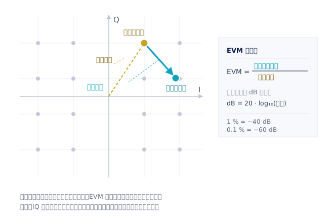
In an ideal world the point received would land exactly on the constellation grid. In the real world it does not. The symbol actually received is a complex vector and the ideal symbol is a complex vector, and the difference between them is the error vector — the short line on the constellation running from the ideal point to the actual one. Error vector magnitude (EVM) is the length of that line, normalised to the amplitude of the reference signal.
Why normalise? Because the absolute length of the error vector grows and shrinks with transmit power, so quoting it directly gives no basis for comparison. Divided by the reference amplitude it becomes a dimensionless ratio, which can be written as a percentage (the error as a percentage of the signal) or in dB. The two are the same thing written twice: the dB value is 20·log10(ratio), so 1% is −40 dB, 0.1% is −60 dB, −45 dB is about 0.56% and −53 dB about 0.22%. By convention, poorer EVM figures (the output of a power amplifier, say) are usually given as percentages and better ones (the residual value of a signal source) in negative dB, because the numbers read more easily that way.
RMS and peak: one number, two questions
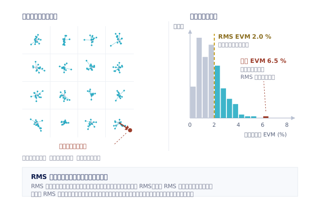
A single measurement captures thousands of symbols, each with its own error vector. The commonest way to condense them into one number is the root mean square (RMS): square every symbol's error, average, take the square root. RMS EVM answers 'how clean is the signal overall', and it is the value quoted by the great majority of data sheets and standard test reports.
Peak EVM answers a different question: 'how bad was the worst single symbol?' The two can tell completely different stories. A signal whose RMS EVM looks healthy while its peak EVM stands out usually means the problem is occasional rather than general — the waveform peak hitting the amplifier's compression region, the start of a burst not yet settled, or intermittent interference. When interpreting, use RMS to see the overall margin, and peak together with 'which symbol, and which quadrant of the constellation' as the clue to the root cause.
There is one more detail, often overlooked, that decides the size of the number: what the reference is. EVM is the deviation of the actual constellation from the ideal one, and that ideal reference does not come out of nowhere — the analyser first has to demodulate the signal, decide which point each symbol was supposed to be, reconstruct an ideal waveform according to the rules of that modulation standard, and only then subtract symbol by symbol. The denominator of the normalisation is a choice as well: some definitions divide by the average power of the reference constellation, others by the peak power of the outermost symbols, and the two do not produce the same number. Most standards also allow the analyser to estimate and remove certain systematic errors before the calculation (carrier frequency offset, sample timing, common phase error). That is why the same signal measured by the measurement applications of different standards gives different EVM figures — before comparing values, make sure both sides used the same set of definitions.
What ruins EVM in a real transmitter
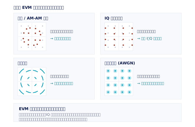
EVM's value is that it is a general ledger: any mechanism that moves the received point away from its ideal position ends up in the same number. Read the other way, the shape of the error on the constellation often reveals the cause (see Fig. 2).
First is power amplifier compression and non-linearity. As an amplifier approaches saturation its gain is no longer constant, and large-amplitude symbols are compressed more than small ones (AM/AM distortion) while the phase also shifts with amplitude (AM/PM distortion). On the constellation this appears as the outer symbols being pulled inward and rotated, while the inner ring stays relatively normal. It is also why EVM almost always degrades as output power rises, and why OFDM signals with a high peak-to-average power ratio (PAPR) are especially sensitive.
Second is IQ imbalance. If the gains of the I and Q paths are unequal, the constellation is stretched into an ellipse; if the two paths are not exactly 90° apart, it is sheared into a rhombus. IQ imbalance also produces an image signal on the other side of the carrier.
Third is local oscillator leakage, that is, carrier leakage. A DC offset in the mixer or baseband lets some unmodulated carrier leak straight through to the output, which is equivalent to adding a fixed DC offset to every symbol on the constellation — the whole constellation is translated away from the origin.
Fourth is phase noise. Short-term phase instability of the local oscillator makes every symbol jitter in the angular direction, and the constellation points blur along an arc (in the tangential direction). This one is particularly lethal to high-order modulation: 256QAM has far tighter decision boundaries than QPSK, so angular jitter that is nearly harmless in QPSK can cause outright bit errors in high-order QAM. It is also why the phase noise specifications of analysers and signal sources are treated as a precondition for EVM performance.
Fifth is frequency error. If the transmit and receive carrier frequencies do not agree, the constellation rotates continuously with time; residual sampling clock error makes the error accumulate progressively with symbol position. Most standards' EVM definitions allow part of this to be compensated first, but whatever remains after compensation shows up directly in the value.
Why standards set an EVM limit
Modulation standards (5G NR, Wi-Fi, LTE and the rest) all set an EVM limit for the transmitter, usually graded by modulation order — the higher the order, the tighter the limit. The reason goes back to the constellation: for the receiver to read a symbol correctly, that symbol has to land inside the correct decision region. The distance between constellation points is the budget available, and that budget has to absorb channel noise, multipath fading, the receiver's own impairments, and the share of the error the transmitter has already spent.
In other words, a transmitter's EVM eats directly into the receiver's demodulation margin. A transmitter with poor EVM may still pass over an ideal laboratory connection, but out in a real environment with a weaker signal and more interference the available margin has already been spent on itself, and the result is reduced receive sensitivity, a forced drop to a lower data rate, and shorter range. A standard sets a limit essentially to guarantee that 'the transmitter may occupy at most this much of the budget', so that the system's link budget can be designed at all.
Note that the details of the EVM definition differ between standards: the basis of the normalisation, which errors may be compensated beforehand, the time range and resource units over which it is averaged, and the power points at which the measurement must be performed are all written into the respective specifications. So 'what is this device's EVM' is an incomplete question unless it names the standard, the modulation and the bandwidth setting it refers to. In practice, conformance decisions should follow that standard's measurement application and the text of its specification, and values should not be compared across standards.
How EVM is actually measured
Measuring EVM takes a vector signal analyser (VSA), not a spectrum analyser that only looks at power. The difference is that a VSA preserves the signal's I/Q waveform — it down-converts the RF signal and digitises it into an I/Q data stream, then performs symbol synchronisation, carrier and clock recovery and channel equalisation according to the specified modulation format, decides the value of each symbol, and uses that string of decisions to reconstruct an ideal reference: 'this is what the waveform should look like if the transmitter were perfect'. Finally it subtracts the actual I/Q from the ideal I/Q symbol by symbol to obtain the error vector, and the statistics of that are the EVM.
The procedure has one hard precondition: the analysis bandwidth must completely cover the bandwidth of the signal under test. Where analysis bandwidth is insufficient, subcarriers at the edge of the signal are cut off or attenuated by the instrument's IF filter — and the analyser does not know it did this itself. It records that distortion faithfully into the error vector and reports an EVM that is systematically high and cannot be calibrated away. Modern wideband signals make this very real: a 100 MHz 5G NR carrier, a 320 MHz Wi-Fi channel, or a carrier-aggregated combination raise the bandwidth requirement on the instrument very quickly.
The R&S signal and spectrum analysers are tiered along exactly this axis. The R&S®FSV3000 offers up to 200 MHz of analysis bandwidth, can capture two adjacent 5G NR carriers at once, and achieves better than 1% 5G NR EVM at 28 GHz with a 100 MHz carrier. The R&S®FSVA3000 pushes analysis bandwidth to 1 GHz under the same EVM conditions (with the FSV3-B1001 option) and can capture up to ten 100 MHz 5G NR carriers in one go. The flagship R&S®FSW offers up to 8.312 GHz of internal analysis bandwidth and typical phase noise of −136 dBc/Hz (1 GHz, 10 kHz offset), covering demodulation and EVM analysis with the K70 vector signal analysis and K144/K145 5G NR measurement options. At the volume production and module test end, the R&S®CMP180 handles Wi-Fi 7 and 5G NR FR1 with up to 500 MHz of analysis bandwidth and two independent RF channels (2×VSA / 2×VSG); the R&S®PVT360A integrates VSG and VSA in one chassis with up to 500 MHz of analysis bandwidth, suited to parallel measurement on a production line; and where modulation quality has to be verified under a real signalling procedure, the R&S®CMX500 covers RF and modulation quality measurements for LTE, 5G FR1/FR2 and Wi-Fi 7.
Do not forget the instrument's own EVM
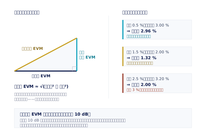
The measurement system has errors of its own. An analyser has a residual EVM, and so does a signal source — when you use a vector signal generator to test a receiver, or to generate the stimulus for testing a power amplifier, the source's modulation quality is the floor of that measurement. Since the errors of the device and of the instrument are mostly uncorrelated, they can in practice be approximated by adding powers: the square of the measured EVM is roughly the square of the device's EVM plus the square of the instrument's.
That relation explains why the instrument has to be 'a class better'. If the instrument's residual EVM is comparable to the device's, the measured value will be noticeably higher than the truth; whereas when the instrument is about 10 dB better than the device, its contribution falls to a negligible level. This is a practical rule of thumb; the actual margin should still be decided by the specification and by an uncertainty assessment.
R&S's vector signal generators are positioned for exactly this. The flagship R&S®SMW200A covers 100 kHz–67 GHz (single path; a dual-path configuration tops out at 44 GHz) with up to 2 GHz of modulation bandwidth, and reaches 0.1% EVM (that is, −60 dB) on 5G NR signals and −53 dB (about 0.22%) on WLAN IEEE 802.11be. The mid-range R&S®SMM100A covers 100 kHz–44 GHz, with EVM better than −45 dB (about 0.56%) on a 400 MHz 5G NR signal at 28 GHz and better than −53 dB on 320 MHz Wi-Fi 7 (IEEE 802.11be); its R&S®SMM-K575 RF linearisation option improves EVM by up to a further 8 dB while raising output power — particularly valuable where a power amplifier has to be tested at a high power point.
One last reminder: EVM is a relative measurement, and its credibility rests on the instrument being in the right state. The calibration interval, running the built-in self-alignment, and compensating for the loss of test fixtures and cables all show up in the value. When an EVM reading looks wrong, checking the measurement chain first usually saves more time than suspecting the design first.