
Frequency range: buy the margin for harmonics, not for the fundamental
Frequency range is the first line of the data sheet and the line most often read only halfway. Most people take the highest operating frequency of the device under test and match it to the instrument's upper limit — measuring a 2.4 GHz Wi-Fi module, they pick a 3 GHz instrument. The problem is that one of the commonest jobs a spectrum analyzer is given is measuring harmonics and spurious emissions: the second harmonic of a 2.4 GHz fundamental lands at 4.8 GHz, the third at 7.2 GHz. If regulation or an internal specification requires verification to the third harmonic, a 3 GHz instrument cannot make the measurement at all — this is not a question of accuracy, it is a question of reach. The general rule: set the upper frequency limit to at least three times the highest fundamental, or five times if you need to see the fifth harmonic.
Apply that rule to a real purchase and it bites. Take a Sub-6 GHz 5G module: a fundamental up to 6 GHz with verification to the third harmonic means a requirement of 18 GHz — a whole price class away from the instinctive '6 GHz should be enough'. The check to run: list every device under test you might meet in the next two years, take the highest fundamental among them, multiply by the highest harmonic order you have to verify, and that number is your frequency requirement.
The lower limit matters as well. Most bench analyzers start at 9 kHz or below, which looks like enough for anything; but if what you measure is conducted emissions from a switched-mode supply (conducted EMI measurements start at 9 kHz or 150 kHz), supply ripple, or low-frequency baseband signals, then the lower limit and the noise performance of the low band become real constraints. Handheld instruments usually start higher, an inherent trade-off for their size and power consumption.
Finally, a higher frequency limit is not a free 'more is better' option. Moving up a class is usually not a linear increase in price, and the high bands often need an external mixer or preamplifier option to keep usable sensitivity. The pragmatic approach is to confirm whether the model supports a later frequency upgrade — most R&S analyzers extend frequency and options by software licence or module upgrade — buy what you need today and leave the margin for the day you actually need it.
Resolution bandwidth (RBW): resolve them, and be able to wait
Resolution bandwidth (RBW) is the bandwidth of the analyzer's IF filter, and it decides whether two closely spaced signals blur into one line on screen. The narrower the RBW, the better the frequency resolution and the lower the displayed noise floor as well — a decade less RBW is roughly 10 dB less noise floor. That is why RBW is narrowed when measuring small signals, and why a DANL figure must always be reported together with its RBW.
The cost is sweep time. On a traditional swept analyzer, at a given span, sweep time varies inversely with the square of RBW: a decade less RBW is about a hundred times longer sweep. Take RBW from 10 kHz down to 100 Hz and a sweep that took a few hundred milliseconds may take tens of seconds. That relation is the most direct expression of 'sensitivity versus speed' on a spectrum analyzer, and it is where a production line hurts most. Modern instruments ease it by replacing part of the sweep with FFT analysis, which can cut measurement time at narrow RBW to a tenth or even a hundredth; but what to confirm when choosing is the actual sweep time under the settings you care about, not the fastest sweep rate printed in the brochure.
What matters when choosing is the range of RBW, not whether the function exists. The narrowest RBW decides how fine a structure you can resolve — measuring adjacent channel leakage, observing a phase noise skirt, or separating two signals a few tens of hertz apart calls for 1 Hz or narrower. The widest RBW affects the ability to measure pulses and wideband signals. Check as well whether the 6 dB bandwidth filters for EMI measurements are offered (the 200 Hz, 9 kHz, 120 kHz and 1 MHz bandwidths CISPR prescribes) together with a quasi-peak detector; these are usually part of an EMI option rather than standard equipment.
One common misunderstanding worth clearing up: RBW is not an 'accuracy' setting. What it affects is resolution, noise floor and sweep time; correctly set, the power reading of a continuous-wave signal does not change when RBW changes. What does change with RBW is the reading for noise and noise-like signals, which is exactly why a noise power measurement has to be normalised for bandwidth.
Three different ceilings: DANL, phase noise and dynamic range
DANL (displayed average noise level) is the analyzer's own noise floor with no input signal, and it decides how small a signal you can see in absolute terms. It has to be reported with its RBW (usually normalised to 1 Hz) and with a statement of whether the preamplifier is on — the same instrument can differ by more than 10 dB with the preamplifier in or out. The practical criterion is direct: subtract DANL from the power of the smallest signal you have to see, and keep at least 10 dB of margin if the measurement is to be stable.
But DANL is only the limit when there is no large signal near your signal. When you are looking for something small beside a strong carrier — measuring adjacent channel power, measuring the spectral purity of a local oscillator, looking at the skirt of a modulated signal — what really blocks you is the analyzer's own phase noise. The skirt of the analyzer's local oscillator lands, by reciprocal mixing, exactly where you wanted to look, and this has nothing to do with DANL: narrowing RBW further and switching the preamplifier on will both fail to rescue it. It is also one of the main reasons for the price gap between high-end and mid-range instruments. The definition, units and measurement of phase noise itself have an article of their own on this site, Phase Noise: What It Is, What It Costs, and How It Is Measured.
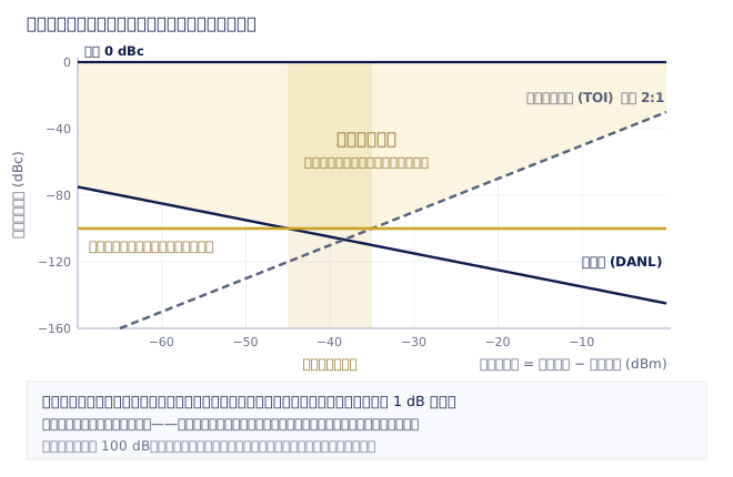
The third ceiling comes from the large-signal end. The higher the input power, the stronger the distortion products the mixer generates: the level of third-order intermodulation products relative to the carriers degrades on a 2:1 slope, usually described by the extrapolated figure called third-order intercept (TOI); above that again is the 1 dB compression point, beyond which even basic readings start to be wrong. So the real operating variable is mixer level — input power minus input attenuation. More attenuation pushes the signal down and you hit the noise floor first; less attenuation and you hit distortion first. The usable measurement window is what the two of them leave in between (Fig. 1).
Once that plot makes sense, it is clear why '100 dB of dynamic range' is a meaningless statement: dynamic range is a window that moves with offset frequency, RBW and attenuation setting, not a constant. Before comparing two instruments, align the conditions — the same offset, the same RBW, the same input attenuation, and the same answer on whether a preamplifier and a low-phase-noise LO option are included — and only then compare numbers. Subtracting two numbers measured under different conditions produces nothing but an illusion.
Analysis bandwidth: the one that decides whether you can demodulate
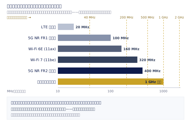
The specifications above are all about how accurately you can measure; analysis bandwidth (also called demodulation bandwidth or real-time bandwidth) is about whether you can measure at all. It is the instantaneous bandwidth the analyzer can digitise in one go and pass to its DSP. To demodulate a modulated signal, compute EVM, display a constellation, or analyse the internal structure of a radar pulse, the signal's entire occupied bandwidth has to fall inside the analysis bandwidth; whatever lies outside is not degraded, it simply does not exist in the captured data.
Comparing that with real standards shows where the thresholds are (Fig. 2): 20 MHz for an LTE channel, up to 100 MHz for a single 5G NR FR1 carrier, 160 MHz for Wi-Fi 6E, 320 MHz for Wi-Fi 7, 400 MHz for a single 5G NR FR2 millimetre-wave carrier, and radar linear-FM pulses routinely above 1 GHz. And margin is needed on top: measurement filters need a window wider than the signal itself, and carrier aggregation, adjacent channel leakage ratio (ACLR) and multi-carrier measurements need more still. Buying an analysis bandwidth exactly equal to the channel bandwidth is usually regretted during the first ACLR measurement.
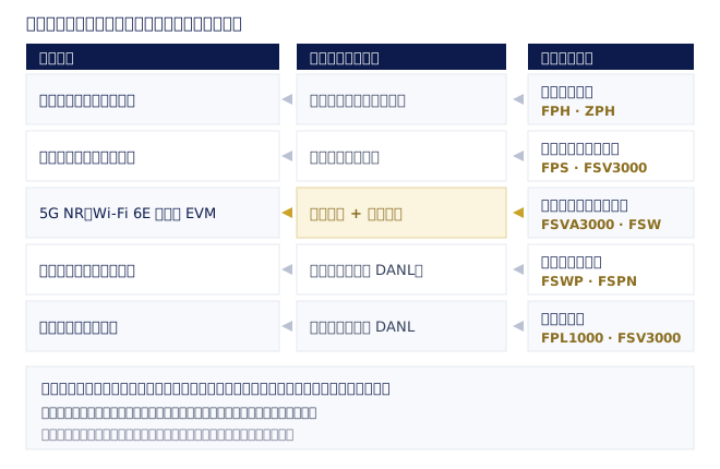
Analysis bandwidth is almost always an option, and one of the most expensive lines on the quotation — at the GHz level its price often exceeds that of the base instrument. This is the moment in a selection that calls for the most honesty: if your work is Sub-6 GHz 5G NR and Wi-Fi 6, a 200 MHz class analysis bandwidth is enough and a mid-range instrument (the R&S®FSV3000, for example) will do it; only FR2 millimetre wave, Wi-Fi 7 or radar pulses call for the high-end class such as the R&S®FSVA3000 or R&S®FSW, which offer hundreds of MHz to several GHz.
A related but different specification is the gap-free capture bandwidth of real-time spectrum analysis, together with the minimum detectable signal duration (probability of intercept, POI). If the job is catching transient, intermittent interference — frequency hopping, bursty packets, coexistence interference — those two numbers matter more than ordinary sweep specifications, and they too are options. Ask about them separately from analysis bandwidth, because the values are often different.
Measurement speed and option software: the real total on the quotation
Measurement speed rises to first place among specifications only on a production line — but once it is first, it outweighs everything else. What a line cares about is total test time per unit: sweep time, the time to switch between settings, the round-trip latency of remote commands, and the repeatability of results — poor repeatability means measuring several times, which lengthens the test by another route. Added together, the differences in these are enough to halve or double the throughput of the same line. Instruments designed for it (the R&S®FPS, for example) deliberately give up some generality in exchange for very short measurement and setup-switching times. In a development laboratory the logic is reversed: for a measurement performed a few times a day, speed is not the point — getting a standard-compliant result at one press is.
And that 'one press' is the option software. A spectrum analyzer's measurement applications (personalities) cover demodulation analysis of all kinds (5G NR, LTE, WLAN, Bluetooth, automotive radar), EMI measurement with CISPR detectors, phase noise measurement, noise figure, pulse analysis, vector signal analysis (VSA) and more. What they have in common is a high unit price and a strong tendency to be left out at the quotation stage — because the cover of the brochure only names the box.
An instrument that looks cheap can, once three or four necessary options are added, total more than a 'more expensive' model that already includes them. So compare configured totals rather than base list prices. This matters especially across brands, because vendors draw the line between standard and optional in different places.
A practical suggestion: before requesting a quotation, write out the measurements you have to perform, one line each — '5G NR FR1 uplink EVM', 'CISPR 32 conducted emissions pre-compliance', 'LO phase noise at 10 kHz offset' — and ask each supplier to mark which hardware and software options each line requires. That table turns two differently formatted quotations into something you can subtract directly, and it also tends to reveal requirements that would be better met by renting or by outsourcing the measurement.
Which class suits which work, and the questions to answer before asking for a quotation
Handheld / field instruments: battery powered, weather-resistant, usable in one hand, for antenna alignment, feeder and VSWR checks, and hunting interference on site. The trade-off is that sensitivity, phase noise and analysis bandwidth all fall short of a bench instrument, and the frequency ceiling is lower. The R&S®FPH and R&S®ZPH belong here. The test is simple: if the measurement has to leave the laboratory, this class is not a compromise but the only workable choice; if the measurement always happens on a bench, do not pay for portability.
Mid-range general-purpose bench instruments: this is the class most laboratories actually need. DANL, phase noise and dynamic range are sufficient for ordinary component verification, harmonic and spurious measurements and pre-compliance testing, with analysis bandwidth usually from tens to a few hundred MHz. The R&S®FPL1000 and R&S®FSV3000 sit in this band, while the entry-level R&S®FPC suits teaching, repair work and basic checks. Honestly: if your work involves no millimetre wave, no ultra-wideband demodulation and no pursuit of extreme close-in performance, buying a flagship only leaves most of its specifications idle inside the case.
High-end signal and spectrum analyzers exist for two things: extremely low internal phase noise, and very wide analysis bandwidth. They are needed for FR2 millimetre wave, Wi-Fi 7, radar pulses, or verifying very clean signal sources. The R&S®FSVA3000 and R&S®FSW are of this class. One distinction is worth drawing: when the measurement target is itself the spectral purity of a source, a dedicated phase noise analyzer (the R&S®FSWP) suits better than a general-purpose analyzer, because cross-correlation takes its effective noise floor to a place a general-purpose instrument cannot reach. There are also models optimised for speed on a production line (the R&S®FPS), and USB / modular analyzers that modularise the RF front end and leave display and computation to a PC — the latter have the lowest cost and smallest footprint and suit automated test racks and multi-channel work, the trade-off being the convenience of standalone operation in the field.
Before asking for a quotation, answer these questions; with the answers in hand the choice very nearly makes itself. One, what is my highest fundamental, and to which harmonic must I verify? Two, how small is the smallest signal I have to see, and at what RBW? Three, is there a large signal next to that small one, and how far away? (This question decides whether you should be comparing DANL or phase noise.) Four, which standards do I need to demodulate, and what is the widest occupied bandwidth? Five, is this development or production, and how many seconds are allowed per unit? Six, do I need EMI pre-compliance, noise figure or pulse analysis? Seven, how many input channels, and is an external mixer needed to extend the frequency? Eight, is this long-term use or a single project? Nine, do the results have to be issued as a traceable report?
The last two questions are really service questions rather than specification questions. A single project does not necessarily have to be bought — taking a high-end instrument on rental and returning it when the project ends is a common and sensible approach, and it is also the best way to verify in practice that an instrument is good enough before placing the order. Long-term use means putting calibration into the annual plan: an analyzer's accuracy drifts with time and temperature, and numbers from an instrument that is not recalibrated on schedule will not stand up in a customer audit or a dispute.