
What a spectrum analyser does: the path from input to trace
An oscilloscope answers the question 'how does voltage change with time'; a spectrum analyser answers 'at which frequencies does the power sit'. The same signal that is an uninterpretable composite waveform on a scope shows at a glance on an analyser where the carrier is, how high the harmonics reach, and whether something is sitting alongside that has no business being there. To read that trace correctly you first have to know how it was drawn — because nearly every setting on an analyser that can make a measurement wrong corresponds to a specific stage of hardware in the signal path.
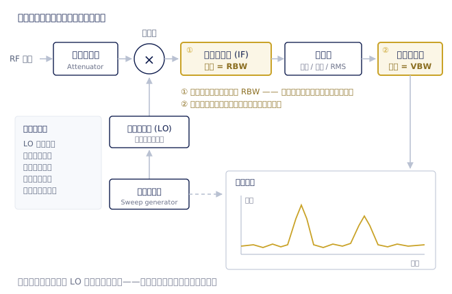
Figure 1 shows the full path of the swept-tuned superheterodyne architecture. The RF signal first passes through the input attenuator (which protects the mixer and also sets the level delivered to it), then enters the mixer, where it is multiplied by the local oscillator (LO). The LO's frequency is driven by the sweep generator, climbing from low to high across the whole span; at any instant, only the signal sitting at 'LO frequency plus or minus the IF' is translated to the intermediate frequency. Once at the IF, the signal passes through a very narrow IF filter — that stage is the physical origin of RBW. After the filter comes the detector, which turns the IF waveform into a number representing amplitude; that is smoothed by the video filter (VBW) and finally drawn on the display.
The line in that diagram that is easiest to overlook and matters most is the one where the sweep generator drives both the LO and the horizontal axis of the display. What it means is that every horizontal position on screen is a moment in time, not only a frequency. The analyser is not watching all frequencies at once; at any instant it sees through a slit exactly as wide as the IF filter. That one sentence leads directly to every trade-off that follows — why a narrow RBW is slow, why sweeping too fast reads low, and why a swept analyser can miss a signal that appears for only an instant.
Resolution bandwidth (RBW): resolving power and noise floor share one knob
RBW is formally defined as the 3 dB bandwidth of the IF filter. Its first effect is intuitive: to separate two signals Δf apart, RBW has to be smaller than Δf. In practice the filter's shape factor matters too (usually stated as the 60 dB bandwidth divided by the 3 dB bandwidth) — a typical Gaussian-shaped filter has a shape factor of about 4.5 to 5. So if the two signals are equal in amplitude, an RBW of roughly Δf will just about show two peaks; but if one of them is 40 dB below the other, the small one hides under the large one's skirt, and you have to drop RBW by a step or more to see it. 'How far apart' and 'how different in amplitude' matter equally, and the amplitude half is the one most often forgotten when choosing RBW.
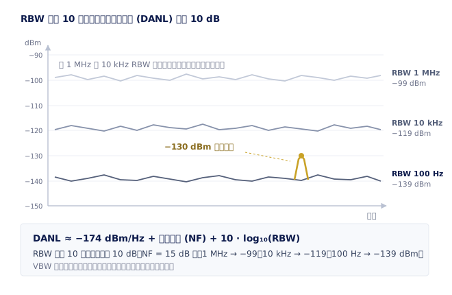
RBW's second effect is to set the noise floor. The noise the analyser displays comes from its own front end: a power density multiplied by the bandwidth that gets through — and what gets through is exactly what the IF filter decides. So the displayed average noise level follows roughly DANL ≈ −174 dBm/Hz + NF + 10·log₁₀(RBW). Take an instrument with a 15 dB noise figure: at 1 MHz RBW the noise floor is about −99 dBm, at 10 kHz about −119 dBm, and at 100 Hz about −139 dBm (Fig. 2). A −130 dBm signal is completely buried in the first two settings, and only surfaces once RBW is down at 100 Hz. When you want to see something smaller, the first knob to reach for is always RBW.
That leads to an extremely practical diagnostic worth committing to memory: change RBW by a factor of ten and watch how the thing on screen reacts. A continuous-wave signal has all its power inside the filter passband, so changing RBW does not change its displayed amplitude — it stays where it is (just narrower). Noise, and noise-like signals much wider than the RBW (a modulated communications signal, say), drop by 10 dB with it. So: 'what falls 10 dB when RBW changes is noise or a wideband signal, what stays put is a discrete signal' — one second of work, worth far more than staring at the trace and guessing.
Most analysers couple RBW to span automatically by default, usually somewhere between 1:100 and 1:1000, which is a reasonable starting point in most situations. Three cases call for manual intervention: separating two closely spaced signals, pushing the noise floor down to see a small one, or meeting a measurement bandwidth that a standard prescribes — EMI measurements, for instance, explicitly require 6 dB bandwidths of 200 Hz / 9 kHz / 120 kHz / 1 MHz rather than the usual 3 dB bandwidth. Those are different filters, and an ordinary RBW cannot stand in for them.
Video bandwidth (VBW) and detectors: where the number on the trace comes from
VBW is often mistaken for 'another kind of RBW', but the two act at completely different points. VBW is a low-pass filter applied after the detector, to the video signal that represents amplitude. What it averages away is the fluctuation of the noise, not the power of the noise. Reduce VBW and you will see a fuzzy noise band converge into a thin line: the reading steadies, and the outline of a small signal buried in noise becomes easier to see. But the average height of that line does not move down; the noise floor is still the noise floor it was. The only way to genuinely lower the noise floor is to change RBW (or lower the noise figure, for example with a preamplifier).
There is a detail here that bites in practice: video averaging on a logarithmic scale is not unbiased for noise. Averaging Gaussian noise logarithmically reads about 2.5 dB below the true RMS power. If you measure the noise power of a channel, or the power of a modulated signal, by 'using a small VBW to flatten the trace', the result is low by that much — and it is systematically low, so taking more measurements will not help. The right approach is an RMS detector with linear power averaging, so the instrument averages in the power domain rather than the log domain.
The detector then decides how each displayed point is picked out of a mass of measurement samples. The display typically has about a thousand points, but the sweep produces far more samples than that, so each displayed point corresponds to a whole bucket of samples, and the detector decides which number represents the bucket. Peak takes the maximum; sample takes whichever sample sits at a fixed position in the bucket; RMS (often labelled average, in the sense of power averaging) averages the power across the whole bucket.
So each detector has a situation in which it lies to you. Peak detection never misses a spur, but it overstates noise — and the wider the span, the more samples land in each bucket and the worse the overstatement; measuring the power of a 5G NR channel with peak detection can read several dB high. Sample detection gives an unbiased noise reading, but it can miss a spur narrower than a bucket entirely, which is particularly dangerous during a spurious search. RMS detection gives the correct power for noise-like and modulated signals and is the only right answer for channel power, occupied bandwidth and ACLR, but it averages away the peak of a narrow pulse. The conclusion is simple: ask first whether this measurement is about 'is it there' or 'how much power', and then choose the detector.
The sweep time square law, and why FFT gets around it
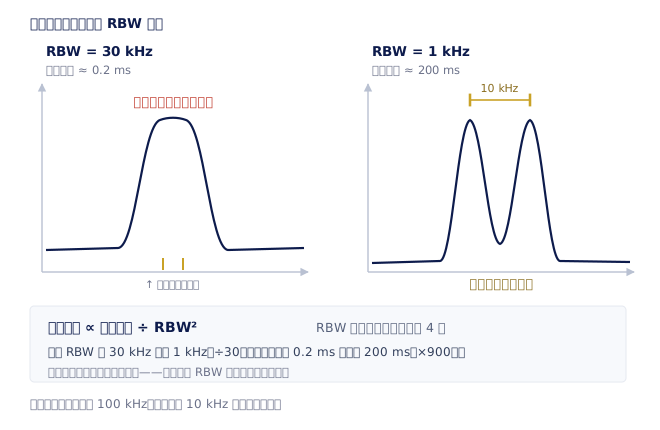
Since the analyser at any instant sees only a slit as wide as the IF filter, there is a lower bound on sweep time. A filter of bandwidth B takes roughly 1/B to settle; as the LO sweeps past each RBW-wide slit it has to dwell at least that long for the filter output to rise to the right height. There are Span/RBW such slits across the span and each needs about 1/RBW, so sweep time T ≈ k · Span ÷ RBW². The constant k depends on the filter type and is of order 1 to 3. The thing to notice in that expression is the square: halve RBW and the sweep takes four times as long.
Figure 3 gives a concrete example. A 100 kHz span with two equal-amplitude signals 10 kHz apart: at 30 kHz RBW they merge into a single hump, entirely unresolved, but the sweep takes only about 0.2 ms; drop RBW to 1 kHz and the two signals separate cleanly, but the sweep stretches to about 200 ms — 30 times less RBW, 900 times the time. Resolution cannot be bought with money, only with time. That is also why narrow-RBW measurements are so painful on a production line: a badly planned full-band spurious sweep can easily run to tens of minutes. Incidentally, if you force the sweep time down, the analyser will usually display a warning such as UNCAL; the filter then has no time to settle, signal peaks are flattened and shifted in the sweep direction, and both the amplitude and the frequency you read are wrong.
Modern analysers sidestep the square law with FFT analysis. Instead of sweeping one narrow filter slowly across the span, a whole block of the IF signal is digitised and a fast Fourier transform computes the spectrum of the entire block at once — which amounts to having thousands of narrow filters side by side. The time required is then roughly proportional to 1/RBW rather than 1/RBW², often one to two orders of magnitude faster at narrow RBW. But FFT is not a cure-all: the bandwidth a single FFT can cover is limited by the instrument's IF and ADC bandwidth, so a wide span still has to be stitched together in segments, and with a wide RBW over a large span a conventional sweep may well be faster — which is why most instruments choose automatically by default. Note as well that swept mode and ordinary FFT mode can both miss an occasional transient: guaranteeing probability of intercept takes a model with gap-free real-time analysis, which is a specification of a different order and has to be confirmed separately when choosing an instrument.
Noise floor is not dynamic range: mixer level, 1 dB compression and TOI
Many people treat DANL as the single measure of an analyser's quality, but DANL is only the lower edge of dynamic range. The upper edge is at the other end: where the mixer starts to distort. What decides that is the level delivered to the mixer, which is the input level minus the input attenuation. And the input attenuator is usually coupled automatically to the reference level — raise the reference level and attenuation increases, the noise floor rises with it but distortion falls; lower the reference level and attenuation decreases, the noise floor comes down but the mixer approaches compression. On an analyser, in other words, 'how small can I see' and 'how large can I measure accurately' are two ends of the same knob.
The upper edge has two concrete numbers. One is the 1 dB compression point: above a certain mixer input level the displayed amplitude starts to read 1 dB low, and on many models mixer 1 dB compression sits somewhere around −10 dBm. The other is the third-order intercept (TOI, also written IP3): when two signals enter the mixer together, non-linearity generates third-order intermodulation products such as 2f₁−f₂, whose level rises with mixer level on a 3:1 slope. The useful relation is that internally generated third-order products sit about 2 × (TOI − mixer level) dB below the signals. For example, with a TOI of +15 dBm and a mixer level of −20 dBm, internal third-order products land about 70 dB below the signals; lower the mixer level another 10 dB to −30 dBm and they drop below 90 dB — but the noise floor has risen 10 dB at the same time.
Draw both of those lines on one plot and you see it: the noise floor gets worse as attenuation increases, distortion gets worse as attenuation decreases, and there is necessarily an optimum mixer level in between. The 'dynamic range' figure printed in a data sheet is normally the value at that optimum, and it is measured at a stated RBW. Which is why comparing two instruments on DANL alone, or on TOI alone, gives a skewed conclusion — either read the manufacturer's dynamic range chart, or work it out yourself with the relation above at the signal levels you actually care about. For harmonic measurements the figure to look at is the second harmonic intercept (SHI) instead, because second-order products rise on a 2:1 slope and behave differently.
Finally, a check that takes thirty seconds and gives a definite answer: when you suspect that a spur on screen is one the analyser produced itself, add 10 dB of input attenuation. A genuinely external signal will not change its displayed level (the instrument compensates for the attenuation automatically); an internally generated third-order intermodulation product falls about 20 dB; an internally generated second-order product falls about 10 dB. If it fell, the problem is not the device under test — you put too large a signal into the mixer. This should become muscle memory: a fair proportion of 'the customer's product has a spur' cases turn out in the end to be a measurement setup problem.
How to choose: when a mid-range instrument really is enough
Honestly: most day-to-day work does not need a flagship. Transmitter harmonic and spurious checks, occupied bandwidth, channel power, ACLR for the common standards, EMI pre-compliance, noise hunting on supplies and clocks — what these measurements need is steady amplitude accuracy, a low enough DANL and a frequency ceiling that covers the job, and a mid-range instrument is entirely up to it. In the R&S line-up, the R&S®FPL1000 and R&S®FSV3000 class is designed for exactly this kind of work; and if the work happens on site, in an equipment room or under an antenna tower, a handheld R&S®FPH or R&S®FPC is more useful than a bench instrument, because the measurement quality is no worse and you can actually take it with you. Buying an instrument far beyond the requirement usually buys nothing but a longer learning curve on sweep time settings.
There are four situations that genuinely call for a step up, and the criteria for each are clear. First, the signal's instantaneous bandwidth exceeds the analysis bandwidth of a mid-range instrument — measuring a 400 MHz 5G NR carrier, a wideband radar chirp or a frequency-hopping signal, insufficient demodulation bandwidth is simply insufficient, and this is where the R&S®FSVA3000 or R&S®FSW class comes in. Second, the device under test is cleaner than the analyser itself — measure a low-phase-noise source and all you will see is the analyser's own local oscillator, a ceiling no setting can get around; our article ‘Phase Noise: What It Is, What It Costs, and How It Is Measured’ covers the detail. Third, catching occasional, transient signals, which needs real-time analysis and triggering. Fourth, seeing something very small right next to something very large, where what decides the outcome is close-in dynamic range and phase noise, not DANL.
When choosing, pin down just three numbers, each with its conditions attached: DANL at the RBW you will actually use, phase noise at the offset frequency you actually care about, and dynamic range or TOI near the signal level you actually have. Once those three are aligned, comparing two instruments becomes a question with an answer. And do not forget to count the calibration interval in the total cost of ownership — a spectrum analyser's amplitude accuracy drifts over time, and on an analyser that is not recalibrated on schedule the data sheet figures are only an indication.