
Which bandwidth class to buy: decide first what question you are answering
The most expensive field on the purchase order is bandwidth, and the reason it gets filled in wrongly is almost always the same: matching it to the clock speed of the bus. The conclusion first — which bandwidth class you should buy depends on how steep the fastest edge on the board is, not on how many times per second it repeats; a control line that looks slow but is driven by a device with a 500 ps rise time makes demands on the instrument that are completely out of proportion to its clock. How edge speed converts into frequency, why the constant is not 0.35 on some models, and why the value you measure is always slow, are covered in full in this site's Oscilloscope Bandwidth, Sample Rate and Probes; this article is only about how the number affects your purchasing decision.
What multiplier to take is a risk decision, not a technical preference. If the oscilloscope's job is only to confirm that the signal comes out and the timing is right, the money saved by being relaxed about it is real. But the moment the waveform will be used to judge overshoot, ringing or monotonicity, or will be pasted into a shipping report or a customer presentation, take five times. The reason is practical: when bandwidth is insufficient the error is one-directional — it rounds the edge off and shaves away overshoot that genuinely exists, and the direction it errs in is precisely the one that will not make you suspicious. An oscilloscope you did not buy enough of will not raise an error; it will simply hand you an over-optimistic conclusion.
Put numbers in and you usually get two results pointing in opposite directions, and both are worth being pleased about. A data sheet stating a 500 ps edge needs 3.5 GHz after the factor of five — already in the price band of a high-end analysis instrument; if the budget only stretches to an entry-level model, that means this measurement either changes method (verify timing only, and get the shape some other way) or gets an instrument of its own. Conversely, the GPIO edges of many microcontrollers land around 5 ns, which works out at 350 MHz, so a 500 MHz entry-level instrument is already ample and the extra money to go up to 1 GHz will not turn into anything you can see. The real value of this arithmetic lies in that second direction: it gives you grounds not to buy the expensive one.
Nor is more bandwidth always safer, for three reasons, all of which are money. First, the wider the front end the more noise comes in with it, so the noise floor on small signals can be worse than on your old instrument and the extra money earns a negative return. Second, probe prices track bandwidth, and they have to be multiplied by the channel count (see the probe section below); move the mainframe up one class and probes may consume half a machine's budget again. Third, on most models bandwidth is enabled with a licence key: buying the same hardware one class lower and opening it up later when the project genuinely gets there is usually better value than buying the top of the range in one go, and the money in between is still yours in the meantime. Three things are worth asking before you order — how far the upgrade path goes, whether the upgrade is purely software or requires a return to the factory, and how warranty and calibration interval are counted after it.
Sample rate, channels and bits: under what conditions was the catalogue number measured
The trap in sample rate is not the number itself but the conditions under which it was measured. On most models the ADC resources are shared between channels, so the maximum on the front of the catalogue is often only available with half the channels switched on, and what is left per channel once they are all on is buried in a footnote inside the specification tables. The architecture behind this, and the comparative figures for each model, are set out in “Oscilloscope Bandwidth, Sample Rate and Probes”; at purchasing time you only have to do one thing: write down the number of channels you will genuinely have on at the same time, ask the vendor to re-quote the per-channel figure under that condition, and check it still leaves at least 2.5 times headroom over the bandwidth. Two instruments with identical cover numbers can differ by a factor of two in this column.
Channel count should be worked back from the most complicated debugging session on your bench, not from 'leave a few spare'. Two channels are only enough to compare an input against an output; four channels are the practical starting point for embedded and power work, because VIN, VOUT, gate and current fill them immediately. If your work often requires an analogue waveform to be lined up against the state of a whole bus, consider a mixed signal oscilloscope (MSO): 4 analogue plus 16 digital is the most common configuration. Two details must be asked before the quotation here — digital channels have their own sample rate and timing resolution and do not get upgraded along with the analogue channels; and whether the logic probe is included in the quotation, since it is frequently listed on a separate options page.
Bit count is the clearest dividing line between model classes in recent years, and the one most worth paying extra for — provided your measurements really are of the 'something small sitting on something large' kind: ripple on a supply rail, gate ringing on a switching node, and fine distortion inside a full-scale analogue signal all qualify. How the number of quantisation steps decides whether you can see these details is covered in full in “Oscilloscope Bandwidth, Sample Rate and Probes”; when selecting, turn it into a question you can answer: how small is the smallest thing I have to resolve, and how large is the signal it sits on? Once that ratio opens up, an 8-bit instrument can only get by with more gain and post-hoc filtering, while a 12-bit instrument simply shows you — and in power integrity work that difference is usually more noticeable than another class of bandwidth.
But discount the nominal bit count. What really represents resolving power is the effective number of bits (ENOB) — what is actually left after front-end noise and distortion are subtracted, and it falls as signal frequency rises. Two instruments both badged 12-bit can differ by more than one bit at the frequency you care about, so the question to ask is 'what is the ENOB at how many MHz', not to be satisfied with the whole number on the cover. By the same token, high-resolution mode is post-processing that trades bandwidth for bits — very useful for measuring low-frequency ripple, but it cannot turn natively 8-bit hardware into 12-bit. When comparing two instruments, normalise the condition to 'how many effective bits at what bandwidth' before you compare.
Memory depth: work back from the window you must capture, do not compare sizes
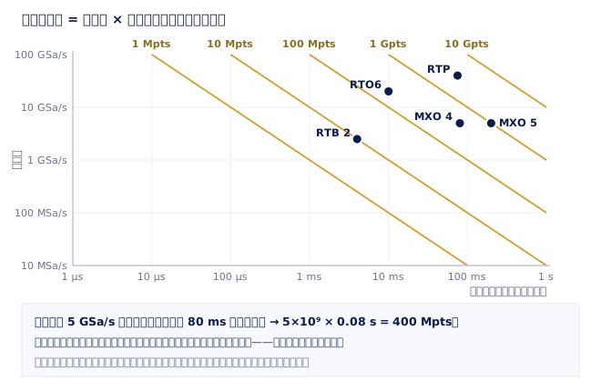
Memory depth is the core specification most easily skipped at the quotation stage and the one most likely to become an obstacle halfway through a project. It is bound together with sample rate and capture window: of the three numbers you may freely choose only two, and the third is fixed by the other two (Fig. 1). “Oscilloscope Bandwidth, Sample Rate and Probes” explains this relationship from the direction of 'how long can this instrument look for'; at purchasing time you use it backwards — write down the longest event you must capture in full, multiply by the sample rate you need, and the resulting number of points is the threshold to put in the specification.
Take a common scenario: capturing an 80 ms boot sequence at full sample rate. 5 GSa/s times 0.08 seconds is 400 million points, that is, 400 Mpts — and that number alone eliminates more than half the candidates. If the instrument to hand has only 10 Mpts, then even backing the sample rate down to 2.5 GSa/s buys only 4 ms; covering the whole 80 ms boot would require the sample rate to fall all the way to 125 MSa/s, and at that density nanosecond-scale edges are long gone from the data. So do not write 'the more memory the better' into a specification; write 'must capture 80 ms continuously at 5 GSa/s' and hand the arithmetic back to the vendor.
The symptom of insufficient memory is silent: the instrument does not tell you it has reduced its own sample rate, there is still a waveform on screen, only the detail has been taken out. So when comparing two instruments, split the question in three — how much ships as standard, how far it can be upgraded, and whether the upgrade is a licence key or new hardware. The third decides whether, two years from now, you make a phone call or budget the purchase all over again. Also make sure you know whether the depth is 'per channel' or 'shared across the instrument': on a shared architecture the depth each channel actually gets with every channel on will be lower than the figure on the cover, the same trap as the channel discount on sample rate.
If the events you are hunting are inherently sporadic — an intermittent fault that shows up every few seconds, a handful of communications packets a minute — then adding memory indefinitely is the most expensive answer, and segmented memory is the right one: it keeps only the fragment around each trigger and throws the blank intervals away. Almost every vendor has the feature, but its usability varies a great deal, and there are three numbers to ask for: how many segments at most, how long each segment can be, and how long the dead time between two segments is. The third is written into catalogues least often and decides success or failure most — if the dead time is too long, sparse events will still slip between your fingers.
Triggering, decoding and update rate: often the real reason you buy one brand over another
The specifications above decide whether you can record the waveform; this section decides whether you can find it. Most of the time actually spent debugging does not go on looking at waveforms but on getting the oscilloscope to stop at the right moment — which is also the area where instruments at the same price differ most and where the difference is hardest to see on a data sheet.
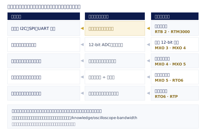
For embedded work, serial protocol triggering and decoding is close to decisive. Whether you can trigger directly on 'a write to I2C address 0x3C', 'CAN ID 0x201 with a particular value in the data' or 'the UART receiving a given character' is the difference between a few minutes and a whole afternoon. Three things to confirm: which protocols are supported (I2C, SPI and UART are the basics; CAN, CAN FD, LIN and FlexRay are automotive; USB, Ethernet, MIPI and SENT are each counted separately); whether triggering and decoding are the same option (some packages give decoding only, with no hardware trigger); and whether decoding is real-time in hardware or post-processed in software — the latter becomes slow enough with deep memory that people give up using it. This is the item most worth trying on your own board before you order.
The waveform update rate (acquisitions per second) determines your chance of catching a rare event. Between two acquisitions the oscilloscope has a dead time, and anything that happens in it is invisible. If an anomaly appears once in ten thousand cycles, an instrument running at ten thousand wfm/s may catch it in seconds while one running at a thousand wfm/s may take several minutes, or by sheer chance may miss it all day. Note that the maximum update rate a vendor quotes is usually taken under specific settings (minimum memory, single channel, decoding off) and will be far lower under real working settings — this too is the item most deserving of verification on a hands-on trial.
What goes with update rate is mask testing and history: let the oscilloscope decide for itself which acquisition violated the boundary you drew, and keep the previous several thousand acquisitions for review afterwards. This is far more effective than a person watching the screen waiting for the anomaly, and it is the key function for turning a rare event into a reproducible problem.
Last come the analysis options: jitter analysis and eye diagrams (high-speed serial links), power analysis (switching loss, safe operating area, harmonics, gate charge), spectrum and FFT analysis (on modern models the FFT is close to a spectrum analyzer in the way it is operated), and the various compliance test packages. As with spectrum analyzers, these options can add up to more than the mainframe itself, so compare 'the total price as configured' rather than the base price of a model number.
Probes: part of the budget, and the ceiling on the whole system
The line most easily skipped on a quotation is the probes, and there are two unwelcome facts about them. First, the measurement capability you have bought is what mainframe and probe come to in series, and it is lower still than whichever of them is worse — put a 500 MHz class passive probe on a 1 GHz mainframe and the system is left at around 450 MHz, so part of what you paid for bandwidth never materialises (the way they combine is in “Oscilloscope Bandwidth, Sample Rate and Probes”). Second, the unit price of a high-end active probe can approach that of an entry-level oscilloscope, and it is not an option but a necessity. The conclusion is simple: compare 'the total price of a configuration that actually works', not the list price of the mainframe.
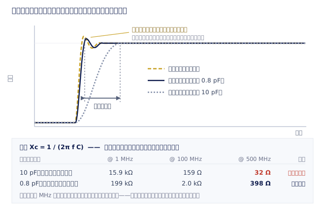
The physics of loading is in “Oscilloscope Bandwidth, Sample Rate and Probes”; for purchasing you only need to remember how it will bite you: once the probe is attached, the edge you measure will be slower than the real one, and the ringing that genuinely exists may instead disappear. Which is to say, what a cheap probe gives you is not 'a worse picture' but 'a better-looking picture' (Fig. 2). That leads to a verification step worth doing: measure the same node once with the probe that came in the box and once with the active probe you are considering, and the gap between them is the amount you would otherwise have misjudged by. Incidentally, switching to a ground spring and using that long ground clip as little as possible is the only improvement on this list that costs nothing.
When selecting, treat probes as a list rather than a tick-box: passive probes for general debugging (the R&S® RT-ZP family); active single-ended probes for high-speed single-ended signals (R&S®RT-ZS); active differential probes for differential pairs and for signals with neither end grounded; high-voltage differential probes for the floating high-voltage nodes of power electronics, and be sure to check their safety category and measurement category really do cover your actual working voltage (the R&S®RT-ZHD family is designed for exactly this); current has to be converted into voltage by a current probe before it can be measured at all; and to see tens of millivolts of ripple on a supply rail you need a dedicated power rail probe (1:1, no attenuation) that pushes the DC level aside with offset compensation and leaves the whole vertical range for the ripple. For extremely high common-mode voltages there are isolated probe systems. Once that list is written out, it is usually the second longest section of the quotation.
Two last places where it is easy to lose out. First, probe quantity has to follow channel count: fit a four-channel mainframe with one high-end probe and the other three channels fall back to the level of the supplied probes, so three quarters of the bandwidth you bought never materialises — ask for the total price with 'one per channel' itemised. Second, when measuring power the voltage and current paths have different delays, so a deskew calibration must be run before measuring, or the instantaneous power will be offset as a whole — and again with no warning, just a set of perfectly plausible but wrong efficiency figures. Probes also age and drift, so if you are keeping them long term, schedule them into the annual calibration alongside the mainframe.
Which class suits which work, and nine questions to answer before the quotation
Entry-level general purpose (R&S®RTB 2, R&S®RTM3000): a few hundred MHz of bandwidth, a 10-bit ADC and four channels, usually with a built-in function generator, and options for logic analysis and protocol decoding, at a price and size that suit one instrument per person on the desk. Good for firmware debugging, sensor interfaces and general circuit verification. Honestly, this class is what most embedded teams actually need, and the key is to spend what you saved on the right probes and decoding options — which is much more noticeable than another class of bandwidth.
Mid-range 12-bit models (R&S®MXO 3 and R&S®MXO 4): a 12-bit ADC, a high waveform update rate and deep memory as standard, the sweet spot for power integrity, switch-mode supplies and mixed-signal debugging. The test is simple: if your problem is 'I cannot see the small signal clearly' or 'I cannot catch the anomaly', this class gives the most direct improvement; if the problem is 'the shape of the edge looks wrong', that is the signal to go up in bandwidth instead.
High-end analysis (R&S®MXO 5, and the R&S®RTO6 and R&S®RTP families): GHz-class bandwidth, extremely deep memory, and a complete jitter and compliance analysis ecosystem. Once the work moves into high-speed serial links, eye diagrams and compliance testing, this class becomes necessary — and be prepared for active and differential probes to take a sizeable share of the total budget. There are also battery-powered handheld models (the R&S®Scope Rider RTH), designed for the field, the production line and high-voltage environments, at the cost of lower bandwidth, memory and analysis capability than a benchtop model at the same price.
Answer these nine questions before asking for a quotation and the selection almost makes itself. One, what is the rise time of my fastest edge? (This sets the bandwidth.) Two, how many channels will I have on at the same time day to day, and what is the sample rate under that condition? Three, how long an event must I capture continuously, and how many points does that multiply out to? Four, how small is the smallest signal I need to resolve, and how large is the signal it sits on? (This decides 8-bit or 12-bit.) Five, which serial protocols do I need, and which option covers triggering and which decoding? Six, how rare is the anomaly I am hunting? (This decides update rate and segmented memory.) Seven, which kinds of probe do I need and how many of each, and what are the working voltage and safety category requirements? Eight, do I need jitter, power or compliance analysis options? Nine, is this for long-term use or a single project?
The last question is a service question, not a specification question. When a single project needs a high-end instrument temporarily, obtaining the use of one for a short period is usually more sensible than raising a purchase order, and it is also the most practical way to verify on your own board whether the instrument really is sufficient before you order. If you are keeping it long term, schedule calibration into the annual plan: vertical gain and timebase both drift with time and temperature, results from an uncalibrated instrument will not stand up in a customer audit or a dispute, and that cost should be estimated into the purchase from the start.