
What a frequency standard actually provides
What a frequency standard provides is a frequency axis. When a counter decides whether a signal is 10.000 000 MHz or 10.000 001 MHz, it does so on the time counted out by its own internal oscillator; the horizontal scale on a spectrum analyzer's screen and the carrier frequency a signal generator puts out ultimately trace back to the same oscillator. That oscillator is called the timebase. When you connect an external standard's 10 MHz to the REF IN on the back of an instrument, what you are doing is replacing the instrument's frequency axis wholesale. The usual output forms are a 10 MHz sine wave (5 MHz or 100 MHz in some contexts) and a 1 PPS (pulse per second) signal — the first to align frequency, the second to align epoch.
The effect scales in proportion. If the timebase has a fractional frequency error of 1×10⁻⁸, measuring 10 MHz puts you only 0.1 Hz out, which seems irrelevant; but the same instrument measuring a 10 GHz signal is then 100 Hz out. So the ceiling on 'how accurate an instrument's frequency reading is' is always its timebase, never its resolution. Measurements that require phase coherence between several instruments — radar, Doppler, multi-channel phase comparison, MIMO — absolutely must share one reference: two instruments each running on their own internal timebase will see the phase difference between them walk away over time.
One more pair of words has to be separated first: accuracy and stability. Accuracy is how far the present output frequency sits from nominal, an offset that calibration can pull back. Stability is how long that offset stays put, and calibration cannot fix it. An oscillator that is 2×10⁻⁹ off but extremely steady is far more useful than one that happens to be spot on now and will be 1×10⁻⁸ away in ten minutes — the first can be compensated with a correction value, the second cannot. What you buy when you buy a frequency standard is stability; accuracy is what the calibration laboratory gives you.
The four axes that actually decide the choice
The first axis is short-term stability, universally expressed as the Allan deviation σy(τ), the single most quoted figure being σy(1 s). The standard deviation is of no use here, because oscillator noise contains drift and flicker components: the sample standard deviation does not converge as the record gets longer, the number simply keeps growing with measurement time and carries no comparative meaning, whereas the Allan deviation is computed from the difference between two adjacent average frequencies and does converge for that kind of noise. How the Allan deviation is calculated, and why you should look at the whole σy(τ) curve rather than a single point, is covered in full in this site's article Allan Deviation: Reading Frequency Stability in the Time Domain. The same thing described in the frequency domain is phase noise, and the two convert into one another — see Phase Noise: What It Is, What It Costs, and How It Is Measured. Behaviour below the millisecond is conventionally read off a phase noise curve, behaviour above a second off an Allan deviation curve.
The second axis is long-term ageing: the rate at which an oscillator's frequency drifts monotonically with time, usually expressed as a fractional frequency change per day or per year. Quartz crystals age, because of stress relief at the crystal surface and the migration of trace contaminants, and this cannot be eliminated, only selected and pre-aged against. The typical orders of magnitude run like this: a general-purpose TCXO at the 1×10⁻⁶ per year level, a good OCXO at 5×10⁻¹¹ to 1×10⁻¹⁰ per day and the 5×10⁻⁸ per year level, a rubidium at the 5×10⁻¹¹ per month level, and a caesium with no ageing term at all. The good thing about ageing is that it is predictable — it is a line of roughly constant slope, so a calibration laboratory can give you a drift rate and you can extrapolate and compensate. What is genuinely awkward is the random-walk component, which cannot be compensated.
The third axis is the temperature coefficient, which deserves particular attention in Taiwan: the on/off cycling of laboratory air conditioning, the thermal behaviour inside a rack and the daily swing in ambient temperature often move your frequency faster than ageing does. A bare crystal has a temperature coefficient at the 1×10⁻⁶ level; a TCXO uses a compensation circuit to push that down to 1×10⁻⁷ to 1×10⁻⁶; an OCXO holds the crystal at its turnover temperature in an oven and reaches 1×10⁻⁹ or better; a rubidium falls between 1×10⁻¹⁰ and 1×10⁻¹¹. Two more specifications that are routinely skipped should be asked about at the same time: warm-up, meaning how long after power-up the unit is within specification; and retrace, meaning whether the frequency comes back to its previous value after the unit has been switched off and on again. A standard that has to be recalibrated every time it is moved or loses power is very difficult to live with.
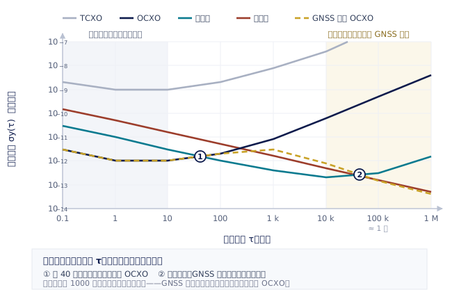
The fourth axis is the combination of cost, size, power consumption and warm-up, and for most projects it is the real constraint. An OCXO reaches specification in a few to a dozen or so minutes, consumes watts, and can be built as a module. A rubidium locks a few minutes after power-up but often needs hours to a day to reach its best stability, consumes tens of watts, and its physics package (lamp and cell) has a service life — it is a component with a finite lifetime. A caesium's beam tube is an outright consumable: when its life is over it has to be replaced, and the replacement costs a significant fraction of the instrument. Lay these four axes out side by side and you will find no single type is best at everything — which is precisely what Fig. 1 is there to show.
The ladder: an honest placing for five kinds of standard
The TCXO (temperature-compensated crystal oscillator) is the default timebase fitted to the vast majority of measuring instruments at the factory, with σy(1 s) around 1×10⁻⁹ and accuracy reckoned at 1×10⁻⁶ per year. Whether you should replace it is, more often than most people expect, no. For timing measurements on an ordinary oscilloscope, general-purpose frequency counting to six digits, or pass/fail decisions on a production line, the accuracy a TCXO provides is far beyond what is needed. Only when the timebase term in your measurement uncertainty budget becomes comparable to the other terms does an upgrade actually buy you something. Put honestly: do the uncertainty breakdown first, then decide whether to spend the money.
The OCXO (oven-controlled crystal oscillator) is the first stop on the upgrade path, and the best value one. A good double-oven OCXO reaches around 1×10⁻¹² at σy(1 s), short-term performance that is in fact better than a typical rubidium. Its weaknesses are all long-term: ageing at the 1×10⁻¹⁰ per day level accumulates to 1×10⁻⁸ to 1×10⁻⁷ over a year, so it needs regular calibration, or somebody watching it. If your measurements all finish inside a minute and you are willing to send the unit out for calibration once a year, the OCXO is often the right answer. The dark blue line in Fig. 1 sitting below every other curve between 1 and 40 seconds is exactly this point.
A rubidium frequency standard locks a crystal oscillator to the hyperfine transition line of rubidium-87. Its σy(1 s) typically falls between 3×10⁻¹² and 1×10⁻¹¹ — which is to say that at the 1 second point it actually loses to a good OCXO, the most counter-intuitive fact here and the one sales talk most often glides past. Its value lies in what happens next: the noise keeps averaging down as τ to the power minus one half, hitting a floor near 1×10⁻¹³ somewhere between a few thousand and ten thousand seconds, while ageing is only at the 5×10⁻¹¹ per month level, two orders of magnitude below an OCXO. In other words, what a rubidium buys you is the stretch from tens of seconds to several months — and it is self-sufficient, needing no antenna, no view of the sky and no external signal of any kind.
A caesium frequency standard sits at the top of the ladder, because the definition of the second is itself the caesium-133 transition frequency. It is a primary standard, in principle requiring no external calibration, with accuracy at the 5×10⁻¹³ level and no ageing term — the reddish-brown line in Fig. 1 that descends at a constant slope and never flattens out anywhere in the observation window is exactly that property. The price is equally plain: cost, size, and a caesium beam tube with a definite service life. In practice the overwhelming majority of company laboratories in Taiwan will never own a caesium; it lives mostly in the national measurement standards laboratory and in telecommunications core sites, and an ordinary laboratory's relationship with it is to be connected to it indirectly, through a calibration report.
The fifth kind is not an oscillator but an architecture: the GNSS-disciplined oscillator. It deserves a section of its own, because it is the most deeply misunderstood of the lot.
GNSS disciplining: you bought the long term, not the short term
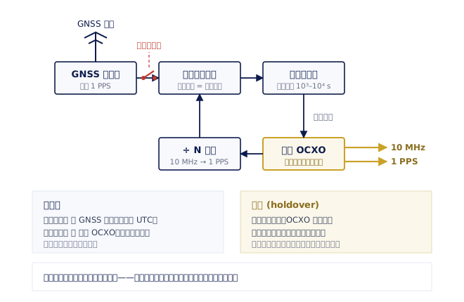
The architecture of a GNSS-disciplined oscillator (GNSSDO) is straightforward, as Fig. 2 shows: the GNSS receiver solves for a 1 PPS, the local voltage-controlled OCXO is divided down to produce its own 1 PPS, the two go into a time interval comparator and are subtracted to give a phase error, and that error passes through a very slow loop filter to become a control voltage that nudges the OCXO. The loop time constant typically falls between 1000 and 10000 seconds — it has to be that slow because the GNSS 1 PPS itself has large short-term jitter (from quantisation error, multipath and the ionosphere), and the loop must average all of that out before it is usable.
And that time constant is the crux of the whole matter: a control loop can only correct errors slower than itself. When the averaging time τ is far shorter than the loop time constant, the loop has no time to respond and the stability of the output is simply that of the OCXO — no better and no worse. When τ is far longer than the time constant, the loop takes over completely, and the long-term accuracy of the output is that of the UTC time scale carried by GNSS, reaching 1×10⁻¹² or better with no ageing. The gold dashed line in Fig. 1 lying exactly on top of the dark blue OCXO line before 1000 seconds is saying just this: the short-term stability of a GNSS-disciplined source is the short-term stability of the oscillator inside its case. So 'this GNSSDO has caesium-grade accuracy' is a statement that only holds at very long averaging times, and taking it as a guarantee of 1 second stability is the most expensive misunderstanding available in this selection.
Rubidium and GNSS disciplining are therefore complementary options rather than competing ones — one holds the middle up, the other pins the far end down. That is also why products of the 'GNSS-locked rubidium reference' kind exist on the market (the Pendulum FTR-210R is one): the short and medium term are handled by the rubidium's atomic transition, the long term by GNSS lock to UTC, and should the antenna lose lock, what takes over in free run is a rubidium with an extremely low ageing rate rather than an OCXO, so holdover is one to two orders of magnitude better. If your requirements include both 'stable at 1 second' and 'no attention needed for a year', that combination is often better value than buying either type alone.
Finally there is installation reality. The long-term accuracy of GNSS disciplining comes with a precondition: the antenna really does have to see the sky. Laboratories in Taiwan are often deep inside buildings, and running the antenna up to the roof means cable routing, lightning protection and waterproofing — engineering cost and subsequent maintenance that are regularly overlooked. Beyond that, the 1 PPS from a GNSS receiver carries a sawtooth error from quantisation, of the order of tens of nanoseconds, and a good receiver will output the correction value alongside it so a downstream stage can compensate — if you intend to use the 1 PPS for epoch comparison, that number has to be asked about. Multipath reflections in an urban environment, and deliberate jamming and spoofing, are also risks to consider at the planning stage, and they are exactly why holdover specifications exist.
How to write a holdover specification, and how to distribute the 10 MHz
Holdover means how long a system can keep itself inside the allowed range once the external reference disappears. It is not a single number but a set of conditions, and the correct way to write it looks like this: 'within 24 hours of GNSS losing lock, with ambient temperature held at 23 ± 3 °C, time error shall not exceed 1.5 µs'. Without the time window, without the temperature condition, without the allowed value, the specification cannot be verified. You can estimate the order of magnitude yourself: an OCXO ageing at 1×10⁻¹⁰/day running free for a day accumulates a few microseconds of time error; swap in a rubidium ageing at the 1×10⁻¹¹/day level and the same day comes out at a few tenths of a microsecond. That is why installations with strict holdover requirements — telecommunications sites, unattended stations — choose rubidium almost without exception.
Two more practical questions belong in the quotation stage. First, when the equipment enters holdover, does it extrapolate using the ageing rate it learned while locked? On models that do, holdover error can be several times better than pure free run. Second, how are you told that lock has been lost? Front-panel indicators, dry contact outputs and SNMP alarms are the three common forms, and if this standard is unattended the alarm interface matters more than the holdover specification itself — if nobody knows it has been unlocked for three days, no amount of holdover will rescue that batch of data.
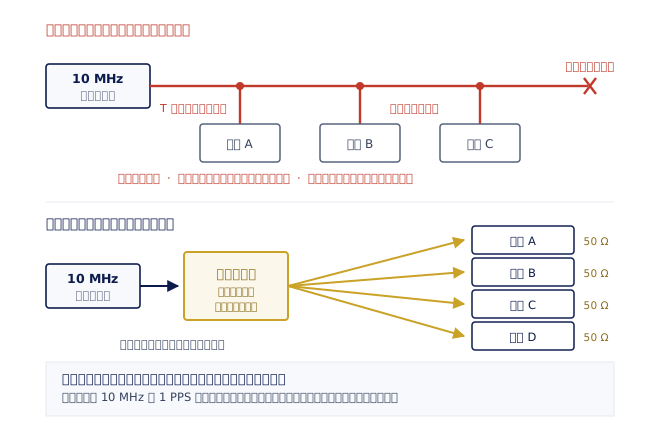
Once the standard is chosen, the next commonly underestimated problem is distribution. A frequency standard usually has only two to four 10 MHz outputs, while a laboratory often has more instruments than that to feed. The most common response, and the one most worth avoiding, is to use tee connectors to daisy-chain one signal to several instruments. Fig. 3 explains why that fails: every tee is an impedance discontinuity and causes reflections; the signal level falls stage by stage along the chain, so an instrument at the end may drop below the minimum input level of its REF IN and quietly revert to its internal timebase; worse still is the coupling — if any one instrument is switched off, unplugged, or changes its own input impedance, the reference for every instrument on the chain moves with it, and none of that movement produces an error message.
The correct approach is a distribution amplifier: the signal goes into the amplifier first and is then sent from several independently buffered outputs, one per instrument, each its own 50 Ω system and isolated from the others. Point-to-point types (such as the Pendulum DA-36) suit sending one signal cleanly to a remote location, while point-to-multipoint types (such as the Pendulum FDA-301) handle the distribution of frequency and time references together. Three things matter when choosing: the number of outputs and the headroom for expansion, the isolation between channels, and whether the amplifier itself degrades phase noise — an amplifier that raises the close-to-carrier phase noise of your 10 MHz by 10 dB has demoted the standard you just bought by one grade. If 1 PPS is to be distributed as well, watch the delay differences between paths and the differences in cable length: those go straight into your epoch measurement results as a systematic error.
Who says your standard is right: traceability, calibration interval and the final decision
Once you have bought a frequency standard you own a claim, but not yet any evidence. The mechanism that turns the claim into evidence is traceability: your standard is compared by a calibration laboratory, that laboratory's reference is compared upward against the national standard, and the chain ends at the SI definition of the second, with an uncertainty and a record at every link. In Taiwan this normally takes the form of a calibration report issued under TAF / ISO 17025. What to read on that report is not just the word 'pass', but the measurement uncertainty, the length of the comparison (an hour of comparison and three days of comparison support completely different statements), and the drift rate relative to the previous calibration — that drift rate is the number you can later use to extrapolate and compensate.
The default calibration interval is a year, but a year is not a law. The sensible approach is to look at the history: if the correction applied at several successive calibrations has been far smaller than your tolerance, the interval can be extended; if one calibration jumps unusually far, the interval should be shortened and you should find out whether the unit was moved, powered down or subjected to an environmental change. GNSS-disciplined models have one extra advantage — while locked they are continuously comparing against UTC, which amounts to self-verification every day; but that only counts if the equipment outputs and retains the comparison records, otherwise you still have nothing to show at an audit. Incidentally, although a caesium standard as a primary standard needs no external calibration in principle, in practice you should still keep records of comparison against other standards, or you will again be unable to demonstrate anything.
Compressing the whole article into one procedure: work back from the application to the averaging time, then pick your line off Fig. 1. Oscilloscope timing and general-purpose frequency counting to six digits — the built-in TCXO is usually enough and no upgrade is needed. Frequency accuracy in RF production test, or a signal generator and spectrum analyzer sharing a reference — an OCXO or a GNSSDO. Radar, Doppler and measurements needing phase coherence at the second level — what matters is σy(1 s), so choose a good OCXO, or check directly whether a rubidium's short-term specification is sufficient. Long-term unattended operation, time stamps and communications applications that must align to UTC — a GNSSDO, with the holdover requirement deciding whether an OCXO or a rubidium sits inside it. Mobile platforms, shielded environments or anywhere with no view of the sky — only a rubidium or a caesium will do, since GNSS cannot help you there.
One last thing: once it arrives, you need to be able to prove it is working. A frequency and time analyzer — the Pendulum CNT-91R, say, or the CNT-104R with its built-in rubidium reference — can compare two standards over a long period and compute the Allan deviation curve directly, showing you which stretch your standard is actually stable over and when it starts to drift. Without that step a frequency standard is a black box you can only believe in and never verify; with it, it becomes a piece of equipment that can stand behind your measurement results.