Why the standard deviation will not do
Suppose you have a 10 MHz frequency standard in front of you, a counter logging a string of readings from it, and you want to describe how stable it is. The instinctive move is to compute the mean and the standard deviation. That is exactly right when you are measuring the length of a steel rule, and on an oscillator it goes wrong — fundamentally wrong.
The reason is an assumption buried inside the ordinary standard deviation (the sample variance): that the random process being measured is stationary and has a finite variance. For white noise that holds — take more samples, get a better estimate, and the number converges on a stable value. But oscillator noise is not only white. It also carries flicker noise (power density proportional to 1/f) and random walk, and the energy of both diverges at the low-frequency end: the lower the frequency the larger the energy, with no lower bound. Compute a standard deviation over a process like that and the result never converges — the longer you measure, the lower the frequency components that work their way into the readings, and the larger the standard deviation becomes.
Numbers make it concrete. The same OCXO might give 2×10⁻¹¹ measured over a minute, 5×10⁻¹⁰ over an hour and 1×10⁻⁸ over a full day. The oscillator did not get worse during that time; all that changed is how much low-frequency drift you swept into the statistic. Which means this 'standard deviation' depends simultaneously on how long you measured and how many points you took, and a different set of measurement conditions gives a different answer. A number that changes with the length of the measurement cannot serve as a specification, and cannot let two vendors be compared fairly.
In 1966 David W. Allan proposed the two-sample variance to solve this, and it went on to become the IEEE and ITU standard time-domain stability measure — today's Allan variance and its square root, the Allan deviation. The insight is really one sentence: do not compare each sample against the overall mean, because the overall mean is itself drifting; compare each sample against its neighbour.
The definition: the difference between two adjacent averages
Start by normalising the measurement. The oscillator's nominal frequency is f₀ and its actual frequency at some instant is f, so define the fractional frequency offset y = (f − f₀)/f₀. It is dimensionless, because the nominal frequency has been divided out, and that is what lets the stability of a 10 MHz standard and a 100 MHz standard be compared directly on the same plot. Average y over an interval of length τ to get the mean ȳₖ of the k-th interval; τ is the averaging time, and it is the independent variable of the whole exercise.
The Allan variance is defined as half the mean square of the difference between adjacent averages: σy²(τ) = ½·⟨(ȳₖ₊₁ − ȳₖ)²⟩, and its square root is the Allan deviation σy(τ). That ½ is not arbitrary — it makes the Allan variance equal the classical variance in the case of pure white frequency noise, so the two agree numerically in the simplest case. Because y is dimensionless so is σy(τ), which is why specifications are written as 5×10⁻¹², 3×10⁻¹¹ and so on, and always with a τ attached: the value at τ = 1 s and at τ = 100 s can differ by more than an order of magnitude, and a stability specification quoting a number without a τ is as meaningless as a phase noise specification quoting dBc/Hz without an offset frequency.
Why does taking adjacent differences rescue convergence? Because differencing two adjacent intervals is equivalent to high-pass filtering the signal: a constant frequency offset is removed entirely and the very low frequency components are heavily suppressed, so the noise processes that diverge at low frequency no longer blow the integral up and the estimate converges. This is also the place to clear up a common misreading: Allan deviation describes stability, not accuracy. A 10 MHz standard that is 1 Hz off will still show a beautiful ADEV provided it is off by a steady amount — stability asks whether the value changes, accuracy asks how far it sits from the true value, and the two are independent questions.
How is it actually measured? You need a reference at least as good as the device under test, or three units compared against one another with the three-cornered hat method used to separate out each one's contribution. The usual arrangement is a counter continuously recording the phase of the device under test relative to the reference as a function of time, from which the ADEV at each τ is computed. There is a trap here that is easy to miss: if there is dead time between consecutive measurements, the signal that fell in the gap biases the result, and the effect is worst at short τ. This is precisely why continuous, zero-dead-time timestamping matters — the continuous timestamping of the Pendulum CNT-91/91R and the gap-free measurement of the CNT-104S and CNT-104R are designed for it, and those models also compute ADEV statistics on board. The counter's own resolution and trigger error land on the short-τ end of the curve as well; for the detail see Frequency Counter Basics: Gate Time, Resolution and the Timebase.
How to read an ADEV plot: the slope is the noise mechanism's identity card
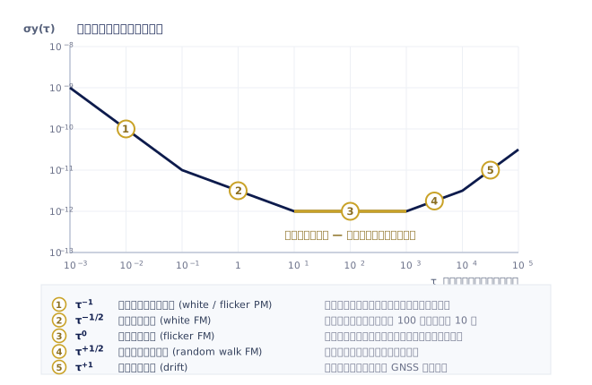
A standard ADEV plot has averaging time τ on the horizontal axis and σy(τ) on the vertical, both logarithmic. Left to right means averaging for longer; further down means more stable. The curve is usually a few near-straight segments joined end to end, and the slope of each segment corresponds directly to one physical noise mechanism — which is what makes the plot so valuable: it tells you not only how stable the oscillator is but why it is not more stable (see Fig. 1).
From left to right: slope −1 comes from white and flicker phase noise, usually contributed by the measurement system itself, by buffer stages and by amplifiers, and it improves in proportion as you lengthen the averaging time. Slope −1/2 is white frequency noise, mostly the thermal noise of the passive resonator; averaging for 100 times as long improves it by a factor of ten. The flat, slope-0 section is flicker frequency noise originating in the resonator itself, and that floor is the stability limit of this oscillator — no amount of averaging will get below it. Slope +1/2 is random-walk frequency noise, which normally corresponds to environmental factors: temperature, supply, mechanical stress, load pulling. Finally slope +1 is linear frequency drift, that is, ageing; for a drift rate D, σy(τ) ≈ D·τ/√2.
In practice there are only three things to look at. First, how high the floor sits — that is this oscillator's limit. Second, at which τ the floor begins and at which τ it ends — that decides whether lengthening the averaging time can buy you the stability you need. Third, how long your application actually averages: if your measurement averages for 100 seconds, then however handsome the curve looks away from the τ = 100 s point, it is not about you. The bumps in a curve speak as well: the time constant of a servo or phase-locked loop usually leaves a bump at the corresponding τ; an oven's temperature cycle leaves one near the cycle period; and a GNSS-disciplined reference shows a knee near the disciplining loop's time constant.
Last comes an honest limitation that is often skipped: the data points at long τ are very unreliable. Estimating the ADEV at τ = 1 day from a three-day run leaves only a handful of independent samples, and the confidence interval is enormous. So when you see a curve drawn from one day of data all the way out to τ = 10⁵ seconds, the reasonable response is suspicion rather than belief. A serious report carries error bars and states the total measurement time; when comparing two sets of ADEV data, ask how long the other party measured before you ask about τ.
Variants: overlapping ADEV, MDEV and TDEV
The most common variant, and the one that should be enabled by default, is the overlapping Allan deviation. The original definition chops the data into non-overlapping blocks, one τ after another; the overlapping form computes the estimate from every possible starting point. The two have the same expected value, but the overlapping form extracts many more samples from the same data, so the confidence interval narrows appreciably and the long-τ points are far steadier. Modern analysis software usually defaults to overlapping, and the report should say so — unless you have a specific reason not to, overlapping is almost always the right choice.
The second variant is the modified Allan deviation (MDEV). As noted above, white phase noise and flicker phase noise both appear with slope −1 on an ADEV plot and cannot be told apart. MDEV inserts an extra layer of phase averaging before the calculation, which separates their slopes (white phase noise becomes −3/2 while flicker phase noise stays at −1), so the noise type in the short-τ region finally becomes identifiable. When do you need it? When the short-τ region is exactly what you care about — qualifying a distribution amplifier or a buffer stage, say, or establishing whether the short-τ section of a curve belongs to the device under test or to the measurement system.
The third is the time deviation (TDEV, σx(τ)), converted from MDEV: σx(τ) = τ·MDEV(τ)/√3. Note that its unit is the second, not a dimensionless ratio — which is exactly the point. In a telecommunications network the engineer does not care about fractional frequency but about how many nanoseconds of time error there are, so the ITU-T synchronisation standards are written in terms of TDEV and MTIE. Pendulum's TimeView™ 3 modulation-domain analysis software provides MTIE and TDEV directly as its two wander analysis measures.
MTIE and TDEV are often used interchangeably, but they measure different things. TDEV is an RMS quantity describing the statistics of the noise; MTIE (maximum time interval error) is a peak quantity describing the largest time error that has occurred within any observation window, which makes it particularly sensitive to a single phase step or switching event. A link can perfectly well pass TDEV and fail MTIE — statistically clean, but it jumped once. Which one to use depends on which standard you are being audited against, and listing both is usually the safest course.
The same thing as phase noise: L(f) and σy(τ)
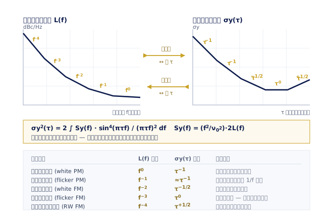
Allan deviation and phase noise are often treated as two independent specifications, but they describe the same set of noise on the same oscillator; only the coordinate system differs. Phase noise L(f) is the frequency-domain description, with offset from the carrier on the horizontal axis; Allan deviation σy(τ) is the time-domain description, with averaging time on the horizontal axis. The two convert into one another through σy²(τ) = 2∫Sy(f)·sin⁴(πτf)/(πτf)² df, where Sy(f) = (f²/ν₀²)·2L(f) (see Fig. 2). That sin⁴ kernel is what 'the difference between adjacent averages' looks like in the frequency domain: a filter that blocks DC and the very lowest frequencies.
The conversion table is worth memorising, and it contains one thing that is easy to get backwards: the two plots run in opposite directions. Far offsets in the frequency domain correspond to short averaging times in the time domain, and close-to-carrier corresponds to long averaging times. The slopes map as follows: white phase noise, f to the power zero, corresponds to τ to the power −1; flicker phase noise f⁻¹ corresponds to roughly τ⁻¹; white frequency noise f⁻² corresponds to slope −1/2; flicker frequency noise f⁻³ corresponds to the flat section; and random-walk frequency noise f⁻⁴ corresponds to slope +1/2. So when somebody says 'this one has a high flicker floor', they are pointing at the same thing on either plot.
Given that they are the same thing, which should you use? The time scale decides. Behaviour below the millisecond, and the effects an RF system cares about — reciprocal mixing raising a receiver's noise floor, the EVM floor of high-order QAM, the jitter of a sampling clock — all live at offset frequencies above 1 Hz, where phase noise is both the natural description and the one that can be measured accurately (see Phase Noise: What It Is, What It Costs, and How It Is Measured). From seconds to days it is the other way round: describing τ = 1 day in terms of phase noise would mean measuring down to a 10⁻⁵ Hz offset, which is not achievable in practice, and there the Allan deviation is the right tool. The two are complementary, not competing.
The conversion has limits of its own, and they are worth stating plainly. The integral converges only for certain noise types; linear drift (ageing) has no counterpart at all in L(f), so an ADEV converted from phase noise contains no drift and its long-τ end will be optimistic. The converted result also inherits every limitation of the original measurement, particularly the upper and lower bounds of the measurement bandwidth — change the integration band and the σy(τ) that comes out changes with it. In practice a dedicated phase noise analyzer will usually compute the Allan variance directly from phase noise data, while a counter measures in the time domain directly; if the two sets of numbers disagree, the first things to check are the integration bandwidth and the measurement time, not the hardware.
From the curve to the purchase: OCXO, rubidium, GNSS disciplining and holdover
Condensing all of the above into something you can act on takes two steps: pin down the τ your application cares about, then compare specifications at that τ. Where does τ come from? A production frequency test with a 1 second gate makes τ 1 second; holding coherence for 100 seconds through a single satellite pass makes τ 100 seconds; a calibration laboratory issuing a report on a 24-hour average makes τ 86400 seconds; and a system required to keep its time error inside some bound for 8 hours after losing GNSS is asking about the holdover specification instead. Until τ is pinned down, no discussion of which unit is better has an answer.
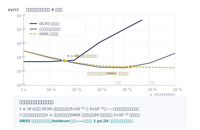
Once τ is fixed, the ranking of the three reference types produces a result that surprises a lot of people (see Fig. 3). Take the actual specifications of the Pendulum 6688/6689: the 6688, built around an SC-cut OCXO, has a short-term stability of 5×10⁻¹² at both τ = 1 s and τ = 10 s; the 6689, built around a rubidium clock, gives 3×10⁻¹¹ and 1×10⁻¹¹ under the same conditions. In other words, at τ = 1 second a good OCXO is nearly an order of magnitude cleaner than the rubidium. Short-term stability is a crystal problem, not an atomic one — the value of an atomic clock lies in the medium and long term: the 6688 ages at 3×10⁻⁹/month and 2×10⁻⁸/year, while the 6689 ages at 5×10⁻¹¹/month and accumulates no more than 1×10⁻⁹ over ten years. The two curves cross at a τ of some tens of seconds, and only past that crossing does the rubidium start to win.
Go further out in τ and ageing becomes the common enemy of both, which is where GNSS disciplining enters. A GNSS-disciplined reference uses the caesium clocks aboard the satellites as its long-term reference and continuously pulls the local oscillator back, so long-term frequency accuracy no longer degrades with age. The actual numbers: the GPS-12R, a GPS-disciplined rubidium, is better than 3×10⁻¹¹ at τ = 1 s, better than 5×10⁻¹² at τ = 100 s and better than 2×10⁻¹² at τ = 24 h while locked; the GPS-88, whose local oscillator is an OCXO, holds its 24-hour average frequency offset better than 2×10⁻¹² when locked to GPS, and continuously compares the local oscillator against the GPS signal, storing the deviation in non-volatile memory so that a traceable calibration report can be printed at any time with GPSView™. Note that GNSS does almost nothing for short τ — short τ is still set by the local oscillator, which is why GNSS-disciplined models still have to be divided into OCXO and rubidium versions.
Last comes holdover, the behaviour after GNSS is lost. It is a separate number and cannot be replaced by the locked ADEV. A GNSS-disciplined rubidium frequency and time reference such as the FTR-210R specifies 1 pps to UTC better than 10 ns rms, typical holdover drift of 1 µs per 24 hours, and an ageing rate better than 5×10⁻¹¹/month in manual holdover mode. Reading a holdover specification means asking three things: for how long, how much accumulated time error is allowed, and under what temperature conditions — because during holdover the dominant error term is usually the temperature coefficient rather than ageing, and a holdover specification with no temperature condition stated is worth almost nothing. For calibration laboratories in Taiwan there is one more practical consideration: GNSS disciplining together with an independent documented frequency comparator (the FTR-210R's Option 220, for example) means traceable reports can be produced in house at any time, rather than shipping the standard out for calibration every year. If multi-channel analysis is needed at the same time, the CNT-104R combines a rubidium clock and a four-channel gap-free analyzer in one instrument, reaching 1×10⁻¹² on a 24-hour average with the GNSS option and a time calibration uncertainty better than 10 ns rms.