
What a counter actually counts: the gate, the ±1 and resolution
What a frequency counter does is, stripped down, very simple: open a gate, count how many times the signal under test crosses the trigger level during the known length of time the gate is open, and when the gate closes divide the count by the gate time to get the frequency. This most primitive approach is called direct counting, it has been in use since the days of mechanical counters, and conceptually there is nothing difficult about it. What is difficult is where its error comes from.
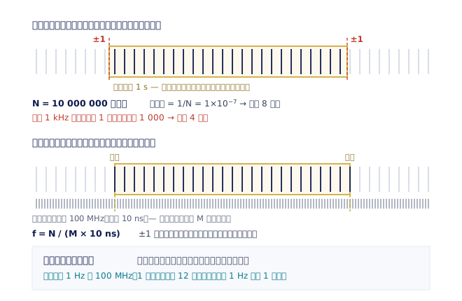
The problem is that the gate and the signal under test are two unrelated things. The gate is generated by dividing down the counter's internal timebase, while the signal under test comes from the outside world, and the two have no synchronous relationship at all. So the instant the gate opens will almost never coincide with an edge of the input signal, and the same goes for the instant it closes. The result is a fragment of a cycle at each end of the gate which may be counted or missed — this is the ±1 count error, a quantisation error no amount of better circuitry can remove (see Fig. 1).
Put numbers in and it becomes obvious. Measure 10 MHz with a 1 second gate and the count N is 10,000,000, so ±1 corresponds to a relative resolution of 1×10⁻⁷, which displays as 8 digits, resolving down to 1 Hz. Take the same instrument and the same 1 second gate to 1 kHz and N is only 1,000, so ±1 corresponds to 1×10⁻³ — still resolving to 1 Hz, but that is now a thousandth of the input frequency, only 4 digits. The resolution of direct counting is tied rigidly to the input frequency, and the lower the frequency the worse it gets: measuring a 1 Hz signal with a 1 second gate leaves you 1 digit, which is the same as measuring nothing.
The only way to gain another digit under direct counting is to make the gate time ten times longer. One second becomes ten for one digit, and another hundred for the next. For an occasional measurement during development that may be tolerable, but on a production line, ten times the test time per unit is a cost nobody will accept. Incidentally, the ±1 error and the timebase error are two different things and have to be estimated separately: the total uncertainty is roughly the combination of the quantisation term (1/N) and the relative timebase error, and whichever is larger dominates.
Reciprocal counting: moving the ±1 onto the reference clock
Modern counters have almost universally moved to reciprocal counting, whose insight is to change what gets counted. The gate is no longer a fixed length of time unrelated to the input; instead the user sets an approximate gate time, and both the opening and the closing of the gate are then synchronised to edges of the input signal. That way the gate contains exactly an integer number N of input cycles with not a single fragment left over. The counter simultaneously counts how many reference clock periods M elapse during that real interval, and the frequency is f = N / (M × T_clk).
The crucial change is that the ±1 uncertainty has moved house. It no longer sits on the input signal but on the reference clock. The reference clock belongs to the counter, its frequency is fixed and high, so the quantisation error becomes a fixed amount of time (10 ns for a 100 MHz clock) that has nothing to do with whether the signal under test is fast or slow. Divide that fixed time error by the gate time and you get a relative resolution independent of input frequency — which is the most important property of reciprocal counting.
The practical difference is dramatic. With the same 1 second gate, reciprocal counting gives you 12 digits whether you are measuring 1 Hz or 100 MHz; the Pendulum CNT-90 and CNT-91/91R are specified at 12 digits/s, the CNT-102 and CNT-104S at up to 13 digits/s, with up to 14 digits displayed. This is also why low-frequency measurement — vibration, sensor outputs, mains frequency, slow clocks — is no longer a counter's weak point. The weak point has become something else, which the next two sections deal with.
Reciprocal counting has its preconditions too. It needs the input signal to be sufficiently periodic with well-defined edges for the synchronising circuit to find the gate's start and stop edges correctly; faced with a burst, with severe distortion or with a signal buried in noise, the synchronisation itself will go wrong. Continuous measurement also raises the question of dead time: a traditional counter misses signal between the end of one measurement and the start of the next, whereas the continuous zero-dead-time timestamping of the CNT-91/91R and the gap-free measurement of the CNT-104S and CNT-104R exist so that not one cycle is lost between consecutive measurements — and for jitter, wander and modulation analysis that matters far more than an extra digit.
Interpolation and timestamping: from 10 ns down to picoseconds
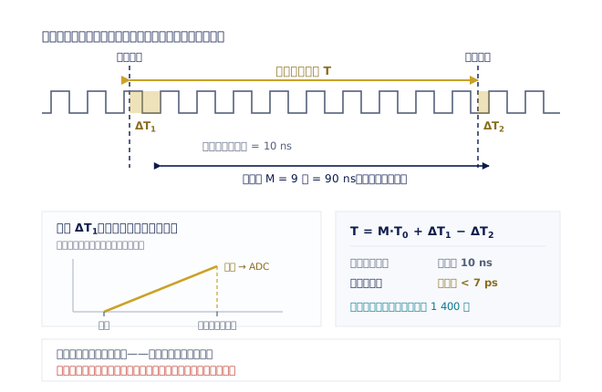
Reciprocal counting moved the ±1 onto the reference clock, but it did not make it disappear. A 100 MHz clock has 10 ns per tick and the coarse count only counts whole ticks; relying on the coarse count alone would leave single-shot time interval resolution stuck at 10 ns, nowhere near enough for measuring PLL lock time, pulse width or jitter. Interpolation is the technique used to slice that one tick finer.
The principle: the start event and the stop event each fall somewhere between two clock edges, so measure the two remainders separately — from each event to the next clock edge — and the true time interval is T = M·T₀ + ΔT₁ − ΔT₂ (see Fig. 2). As for how a remainder is measured, the classic approach is time amplification: the event triggers a linear ramp circuit that starts charging and stops at the next clock edge, at which point the voltage is proportional to that remainder and an ADC measures the voltage — a time difference converted into a quantity that is far easier to measure. There are also implementations based on delay lines or on the vernier principle; the idea is the same.
The effect is immediate. With the same 10 ns clock plus interpolation, the Pendulum CNT-90 achieves 70 ps single-shot timestamp resolution, the CNT-91/91R 35 ps, the CNT-102 14 ps, and the CNT-104S and CNT-104R better than 7 ps — a single tick subdivided more than a thousandfold. Today's high-end models go further still, towards a pure timestamping architecture: every event that crosses the trigger level is given a high-resolution time stamp, and frequency, period, phase and time interval error (TIE) are all derived in software from that one stream of timestamps. This is also where the high throughput comes from — the CNT-90 and CNT-91 reach 250,000 measurements per second, and the internal measurement rate of the CNT-104S reaches 20 million per second.
One point has to be made very explicitly here: interpolation improves resolution, not accuracy. Resolution is how finely a single measurement can discriminate; accuracy is how far the resulting number sits from the true value. The interpolator itself has non-linearity errors that need calibrating, and on a real signal what limits you is often neither the interpolator nor the clock but the trigger noise discussed in the next section.
The ceiling on accuracy is the timebase, not the counting logic
When a counter measures frequency, it is fundamentally comparing the signal under test against its own timebase. So the counter's relative frequency error cannot be smaller than the relative frequency error of its timebase — if the timebase is off by one part per million the reading is off by one part per million, and it makes no difference whether you bought an 8-digit or a 14-digit instrument. The displayed digits beyond the timebase's accuracy are digits with precision but no accuracy: repeat the measurement and it will be very consistent, consistently wrong.
Reading a timebase specification therefore means separating several items that add up. First, the calibration uncertainty at the factory or at the last calibration. Second, ageing, usually quoted as a relative drift per day, per month or per year. Third, the temperature coefficient, quoted as the maximum change across the whole operating temperature range. Fourth, short-term stability, usually given as the Allan deviation at τ = 1 s and 10 s. On top of those come the effects of supply voltage variation, load variation and warm-up time. Take the OCXO in the Pendulum 6688 high-stability frequency standard: calibration uncertainty 5×10⁻⁹ (+23 ±3 °C), ageing 3×10⁻⁹/month and 2×10⁻⁸/year, short-term stability 5×10⁻¹² at τ = 1 s; the 6689 in the same family, built around a rubidium clock, has a calibration uncertainty of 5×10⁻¹¹, ageing of 5×10⁻¹¹/month and total ageing no greater than 1×10⁻⁹ over ten years.
Put those numbers beside the resolution figures from the previous section and the conclusion surprises a lot of people. A 12-digit counter has a resolution of 1×10⁻¹² on a 1 second measurement; but if its timebase is an OCXO that has not been calibrated for a year, ageing alone has already taken it 2×10⁻⁸ away — four orders of magnitude worse than the resolution. Put another way, the last four or five digits are describing the drift of the timebase, not the device under test. That also explains a common observation: two counters of the same model measuring the same signal start to disagree at the 8th digit, which is usually not a fault but two timebases having drifted to different places.
The practical order of business is clear. On entry-level instruments the standard timebase is often a TCXO (the CNT-102, for example, ships with a TCXO at 1 ppm/year, that is, the 1×10⁻⁶ level), an accuracy grade completely out of proportion to 12 digits of resolution; the upgrade option is an OCXO (the CNT-90 offers grades of 0.01 ppm/month and 0.003 ppm/month), and above that sit models with a built-in rubidium clock such as the CNT-91R and CNT-104R. For most laboratories, though, the best value is not a new counter but connecting the counter you already have to a traceable external 10 MHz standard — the 6688/6689 can feed as many as eleven instruments at once, while the GPS-88/89 and FTR-210R use GNSS to lock long-term accuracy directly to UTC. How these numbers should be compared against one another, and what τ makes the comparison fair, belongs to the Allan deviation, which this site covers separately in Allan Deviation: Reading Frequency Stability in the Time Domain.
Trigger level, hysteresis and noise: the errors that are not on the data sheet
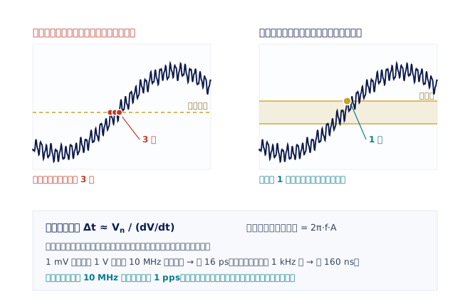
What a counter counts is events, and an event is defined by a comparator at some trigger level: the signal crosses that line going up, and that counts as one. On a clean square wave there is nothing to discuss, but on a real signal there is always noise riding along, and noise makes the signal cross back and forth through the trigger level several times — one real edge counted as three, or five (see Fig. 3).
The remedy is hysteresis: replace the single trigger line with a band, so the signal has to travel all the way from the lower edge of the band to the upper before it counts as one trigger, and small reversals part-way are ignored. The price is that the trigger point is pushed slightly later, and the wider the hysteresis band the larger that delay and the uncertainty it brings. Hysteresis is therefore a parameter to open just wide enough, not as wide as possible.
More fundamentally, trigger noise converts directly into time error, and the denominator of the conversion is the slew rate of the signal: Δt ≈ Vn / (dV/dt). The slope of a sine wave at the zero crossing is 2π·f·A, so the lower the frequency and the smaller the amplitude, the larger the time error the same noise produces. A concrete example: 1 mV of noise on a 10 MHz sine wave of 1 V peak gives a time error of about 16 ps; the same 1 mV of noise on a 1 kHz sine wave gives about 160 ns — amplified ten-thousandfold. That is why, on an instrument with picosecond resolution, the real limit when measuring a low-frequency signal is never the resolution but the trigger noise.
Several practical rules follow. First, when comparing frequency standards use the 10 MHz sine output rather than 1 pps — but not for the reason usually given. A 1 pps pulse has a fast edge, roughly 1 V in 5 ns, a slew rate of 2×10⁸ V/s, which is actually steeper than the zero-crossing slope of a 1 V peak 10 MHz sine (2π·f·A ≈ 6.3×10⁷ V/s), so the trigger error on a single edge is in fact smaller. The real difference is the number of events available to average: 10 MHz delivers 10⁷ edges per second while 1 pps gives you one, and since statistical uncertainty falls roughly as the square root of the number of events, the same gate time differs by a factor of about three thousand — that is the reason frequency standard comparisons are made on 10 MHz. Second, provided the input is not overdriven, turn the signal amplitude up as far as it will go and set the trigger level where the waveform is steepest (the mid-point, for a sine wave). Third, when measuring a slow or noisy signal, switch on the input low-pass filter and open the hysteresis up a little. Fourth, watch the input specifications themselves: the CNT-90's sensitivity is 15 mV rms (to 200 MHz) and 35 mV rms (at 400 MHz), and the CNT-102's input switches between 1 MΩ/40 pF and 50 Ω — pick the wrong impedance and what you measure is the reflection off the cabling, not the device under test.
Beyond frequency: what else it can measure, and an honest account of what it cannot
Once the architecture becomes 'every event carries a time stamp', the quantities that can be derived go well beyond frequency. Common functions include period, time interval (start on channel A, stop on channel B), pulse width, rise and fall time, duty cycle, the phase difference between two signals, frequency ratio, totalising, time of flight, and the time interval error (TIE) that communications and synchronisation work cares about. Microwave models add another layer: the CNT-90XL reaches 27, 40, 46 or 60 GHz and can be optioned with pulsed RF measurement (pulse widths down to 30 ns, including PRI/PRF, burst frequency and burst power), a combination used in radar and satellite communications testing.
The other large category is statistics and the modulation domain. A counter can give you mean, maximum and minimum, standard deviation and Allan deviation on the spot, and present the distribution as a histogram or a trend plot; plotting frequency against time is modulation domain analysis (MDA), which fills the gap between the oscilloscope (voltage against time) and the spectrum analyzer (voltage against frequency). VCO settling time, the PLL lock process, FM/FSK frequency deviation, frequency hopping, chirp and Doppler shift are all seen most clearly in this domain. The CNT-102 and CNT-104S have MDA built in, while the CNT-90 and CNT-91 families achieve it with the TimeView™ software, and TimeView 3 additionally provides wander analysis measures such as MTIE and TDEV.
Next comes the equally important part that data sheets do not print: what a universal counter cannot do. First, it has no frequency selectivity — it measures whichever single signal dominates at the input. If two signals of comparable strength are present at once, or if harmonics, spurious content or noise carry enough energy to capture the trigger, the reading is a meaningless number and nothing on the display will tell you something has gone wrong. Establishing what is actually present at the input is a spectrum analyzer's job. Second, it is not a phase noise analyzer: a counter can give you stability in the time domain (Allan deviation), but a close-to-carrier L(f) curve needs dedicated instruments built on phase detectors and cross-correlation (see Phase Noise: What It Is, What It Costs, and How It Is Measured). Third, it cannot see the shape of a waveform — overshoot, ringing and level anomalies all need an oscilloscope. Fourth, apart from the power measurement on microwave models, it does not measure amplitude at all.
Finally, selection comes down to a handful of questions. How many signals at once? For several devices under test in parallel go straight to the multi-channel models (the CNT-104S and CNT-104R have 4 parallel channels and can measure them gap-free simultaneously). What is the highest frequency? Basic channels are usually 400 MHz, RF options reach 24 GHz, and for microwave look at the CNT-90XL. How much throughput? From 250,000 to 20 million measurements per second are different classes of instrument. Does it need to carry its own traceable reference? If so, look at the CNT-91R or CNT-104R with their built-in rubidium clocks, or feed the whole laboratory from an external standard. Answer those four first and most of the argument over digits on the data sheet settles itself.