
What a signal generator does: the dividing line between analogue and vector
Test instruments come in two roles: analysers look, generators give. A signal generator exists to put a signal known to be right at the input of a device under test — it is the weak source when measuring receiver sensitivity, the swept-level stimulus when measuring amplifier gain and compression, the sweeper when measuring filter response, and the reference when calibrating a whole measurement chain. That role sets its one criterion: the generator has to be more trustworthy than the device. As soon as the generator's own imperfections are the same order as the device's, the measurement has no conclusion in it.
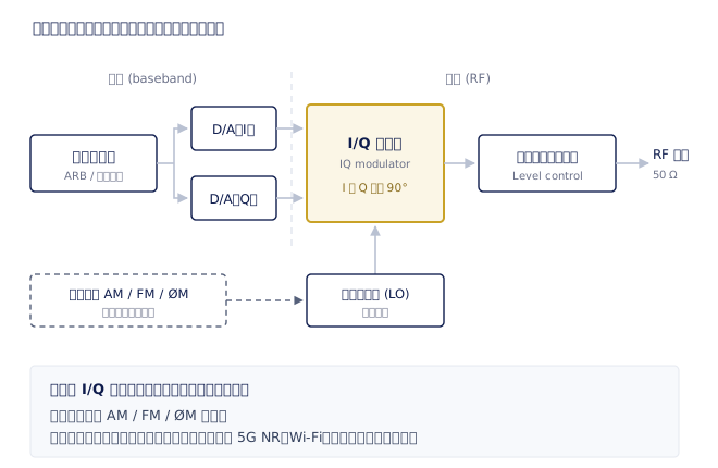
The first fork in the product line is analogue versus vector. An analogue signal generator puts out a continuous wave and can apply amplitude modulation (AM), frequency modulation (FM), phase modulation (ØM) and pulse modulation; it spends its entire budget on frequency range, level accuracy and spectral purity, so at a given price an analogue instrument usually has better phase noise and spurious performance than a vector one, and often a higher frequency ceiling as well. A vector signal generator adds a whole baseband and I/Q chain ahead of the carrier path (Fig. 3), and can generate any complex signal described by an I and a Q component — every digital communications standard, radar waveforms, even channel simulation with fading and noise added, are all produced on that path.
Two other things to settle when choosing usually decide the price class earlier than 'analogue or vector' does. One is frequency range, especially the upper limit — within one model family, going from 6 GHz to 20 GHz or 40 GHz often costs more than a complete set of modulation options, so be clear first about how many GHz you genuinely have to reach, including whether you have to see harmonics. The other is both ends of the output level range: driving a power amplifier or a mixer is about maximum output power, while receiver sensitivity work is about the lowest usable level (often −120 dBm and sometimes −140 dBm) and about the accuracy at that level — which is the harder end to build.
CW output: what the device receives is not the level you see on the display
Frequency first. The frequency resolution of a CW output on a modern instrument is usually finer than 0.001 Hz and is never the problem; what actually decides frequency accuracy is the internal reference oscillator. The standard fit is usually a TCXO, with an ageing rate of the order of 10⁻⁶ per year; better absolute accuracy means adding an OCXO option or locking the instrument to an external 10 MHz reference. If a test system contains several instruments, locking them to one reference is not only about accuracy but about keeping their frequencies from drifting relative to each other — a precondition for any phase-coherent measurement.
Then level accuracy, where two ideas are often conflated. Absolute accuracy is 'when I set −10.00 dBm, what is really at the output connector', typically specified at ±0.4 to ±0.9 dB and degrading near the top of the frequency range and at very low levels. Repeatability is 'when the same instrument goes from −10 dBm to −11 dBm, is that 1 dB really 1 dB', and that number is usually far better. Relative measurements such as compression point and gain flatness in fact depend on repeatability; absolute accuracy only enters when you report absolute power. Watch the switching points of the internal step attenuator as well — the level takes a small step as it crosses one, and a level sweep that happens to straddle a switching point can look like an anomaly in the device under test.
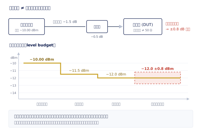
But even with ±0.4 dB of absolute accuracy, the level reaching the device can still be several dB different, because the specification is guaranteed only at the plane of the output connector. Figure 2 lays out what happens in between: 1 to 2 dB of loss in an ordinary coaxial cable at a few GHz is quite normal, an adapter takes a few tenths more, and the least intuitive item is impedance mismatch. Neither the generator output nor the device input is a perfect 50 Ω, and the two reflections act back and forth to produce a ripple that varies with frequency. The rough estimate is ±20·log₁₀(1 ± |Γs|·|Γl|): with a generator VSWR of 1.5 (|Γ| ≈ 0.2) and a device VSWR of 2.0 (|Γ| ≈ 0.33), the product is 0.066 and the ripple is about ±0.55 dB — and it swings up and down with frequency, so it is not a fixed offset you can subtract.
There are three levels of remedy, in order of trustworthiness. The most reliable is to measure with a power meter at the device's own plane and treat that reading as the truth. Next is to sweep the loss of the whole chain once with a power meter and write the result into the generator's user correction table, so the instrument compensates automatically by frequency — particularly worthwhile for automated tests that sweep many frequency points. The least effort, though it has a price, is to put a well-matched fixed attenuator (6 or 10 dB, say) at the device end to suppress the mismatch ripple: add a 6 dB attenuator and the product of the reflection coefficients falls another 12 dB, so the ±0.55 dB above shrinks to about ±0.14 dB. The price is 6 dB of usable level — accuracy traded for dynamic range, and whether that is worth it depends on the application.
Modulation: from AM / FM / ØM to I/Q and ARB playback
The three basic forms of analogue modulation each have their own specification language: AM uses modulation depth (a percentage), FM uses frequency deviation (Hz), ØM uses phase deviation (radians). The modulating source can be the instrument's internal LF generator or an external input. These apparently antique functions are still heavily used — the test signal prescribed by many receiver sensitivity standards is a carrier with 1 kHz, 30% AM, and FM broadcast and two-way radio testing cannot do without it either. One other function usually grouped on the analogue side but specified quite differently is pulse modulation: for radar and EMC work what matters is the on/off ratio (often required to exceed 80 dB) and the rise time, not modulation depth.
Digital modulation all goes down the I/Q path (Fig. 3). Any complex signal can be decomposed into in-phase (I) and quadrature (Q) baseband waveforms; the I/Q modulator multiplies each by a carrier 90° apart and adds them, synthesising the modulated RF. The difference between QPSK, 256QAM and OFDM is only the trajectory the I and Q components follow. Note that the modulator itself has imperfections — I/Q gain imbalance, quadrature error, carrier leakage — which appear as the generator's residual EVM, and that is why a vector generator's data sheet states a residual EVM value outright. (The definition of EVM, and what each impairment looks like on a constellation diagram, are covered in our article on EVM.)
ARB (arbitrary waveform) is where a vector instrument's real power lies: a pre-computed sequence of I/Q samples is stored in waveform memory and played back seamlessly at a fixed sample rate. Three numbers matter when choosing. Sample rate sets the maximum signal bandwidth (the usable RF modulation bandwidth is in practice up to about 0.8 times the sample rate), and that is the threshold for whether a 400 MHz 5G NR carrier or a wideband radar chirp can be generated at all. Memory depth sets how long a non-repeating sequence you can play — measuring long frame structures, realistic traffic or long-period frequency hopping, insufficient memory leaves you looping the signal. Third is whether real-time coding is available: a BER test needs the device to see continuously changing data, not one fixed frame replayed every few milliseconds.
There is a boundary here that has to be faced honestly: a looped ARB waveform is not real traffic. Receiver conformance testing often also needs real-time signal generation, additive white Gaussian noise (AWGN) and fading channel simulation, and these are almost always chargeable options. Note too that the generator's own residual EVM has to be clearly better than the device's specification — the habit is at least 10 dB of margin, or a good share of the EVM you measure comes from the source.
Spectral purity (1): which measurements phase noise ruins
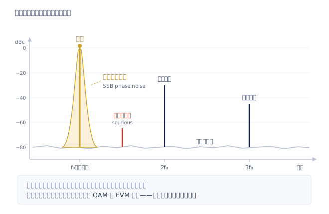
Phase noise is the noise skirt extending continuously outward on both sides of the carrier (the ring in the middle of Fig. 1), expressed in dBc/Hz, and it must be reported together with an offset frequency — the same instrument can differ by more than 30 dB between 10 kHz and 30 MHz offset, so 'this one is −132' is not a specification until the offset is named. Its definition, measurement methods and the cross-correlation technique are covered in full in our article ‘Phase Noise: What It Is, What It Costs, and How It Is Measured’; here we deal only with the direct consequences for a signal generator user.
The classic case, and the one most likely to come off the rails, is receiver blocking and selectivity testing. Such a test puts a very large interferer in a channel adjacent to the receiver under test and checks whether it can still demodulate a weak wanted signal correctly. The problem is that the phase noise skirt of that large interferer extends right into the channel where the wanted signal sits. One calculation makes it clear: interferer at 0 dBm, phase noise at 800 kHz offset of −140 dBc/Hz, receiver channel bandwidth 200 kHz (53 dB), and the noise power smeared into the wanted channel is 0 − 140 + 53 = −87 dBm. If the standard calls for a wanted signal level of −99 dBm, the test simply cannot be performed — what you would be measuring is the generator, not the receiver.
So the rule is hard: at the test offset, the source's single-sideband phase noise has to be at least 10 dB below the threshold the standard implies. The break-even point in the example above is −152 dBc/Hz (0 − 152 + 53 = −99 dBm, exactly the wanted signal level), so another 10 dB means about −162 dBc/Hz to be clean enough — already close to what a top-end signal generator with a low-phase-noise option can do. When the instrument cannot reach it, the industry's standard answer is to put a band-pass or band-stop filter after the generator output and filter the skirt away in the wanted channel. That is entirely legitimate and widely practised; it just means a different filter for every frequency point, which has to be planned for in an automated test.
The second consequence shows up in modulation quality. Integrating phase noise over the offset range of interest gives an RMS phase error, and that value is approximately the EVM floor imposed by phase noise. What nobody worried about in the QPSK era becomes a project killer at 256QAM and 1024QAM, because the denser the constellation, the smaller the phase wander it tolerates. One last reminder: low phase noise is an option rather than standard equipment on most models — on the R&S®SMA100B, for instance, low phase noise, improved close-in phase noise and ultra-low phase noise are separate options, and an OCXO also changes the close-to-carrier part of the curve. When reading specifications, make certain you are comparing the same configuration.
Spectral purity (2): harmonics, non-harmonic spurs and broadband noise
Figure 1 is a complete map of the impairments. Besides the phase noise skirt, three other things appear where they should not, and each ruins a different measurement.
Harmonics land at integer multiples of the carrier, and are usually specified as something like < −30 dBc with a condition attached such as 'below a given output level' — because harmonics get worse as output level rises, and are at their worst with the instrument pushed to maximum power. Their most direct victims are filter stopband measurements and amplifier harmonic measurements: that second harmonic on screen, did it come from the device under test or from the signal source? There is a thirty-second test — lower the generator's output level by 1 dB: if the harmonic falls by 1 dB with it, it comes from the device under test; if it falls by about 2 dB, it is a second-order product generated by the signal generator (or by some stage after it). The cure is a low-pass filter at the generator output.
Non-harmonic spurs are the most dangerous of the four, because they bear no multiple relationship to the carrier and their position cannot be predicted. They come from the fractional-N mechanism of the synthesiser, multiples of the reference frequency, supply ripple and internal digital clocks. A common specification is < −90 dBc with an offset condition. The danger is that one may land precisely in the channel you are measuring, where it looks exactly like an intermodulation product created by the device. To tell them apart, move the carrier frequency slightly: products created by the device move with the carrier in a predictable way (a third-order intermodulation product moves three times as far as the carrier), while fixed reference-related spurs do not follow the same rule.
The broadband noise floor is the flat horizontal section at the far end of the curve, for example −162 dBc/Hz at 30 MHz offset. Its victims are sensitivity tests and desense tests — anything where a strong signal and a sensitive receive band are not far apart in frequency, the transmit/receive spacing of an FDD system being the classic example. To judge it, convert dBc into an absolute value and compare with the receiver's noise floor: a 0 dBm carrier with −150 dBc/Hz broadband noise injects −150 dBm/Hz into the receive band; over a 10 MHz bandwidth (70 dB) that is −80 dBm, enough to cost a good receiver its sensitivity. When reading a specification, first check whether the manufacturer states a relative value (dBc/Hz) or an absolute one (dBm/Hz), and convert it once at the carrier level you will actually use. If it is not enough, the answer is again an external filter.
How to choose: when a CW source is enough, and when only a vector instrument will do
Start with the cases where it is enough, because there are more of them than people expect. As a substitute local oscillator, a mixer drive source, a clock injection source, a swept stimulus for filters and amplifiers, a power reference for a measurement chain, or for traditional receiver tests needing only AM / FM / pulse modulation — this work calls for frequency range, level accuracy and purity, and a good analogue CW generator is not only sufficient but will have better purity than a vector instrument at the same budget. The R&S®SMB100B is the typical choice in this position; when the measurement needs better phase noise and level accuracy, or has to extend into the microwave bands, step up to the R&S®SMA100B class.
The cases where only a vector instrument will do are equally clear: as soon as the device is a transceiver for any digital communications standard, or the measurement is EVM, ACLR or receiver conformance testing, you need I/Q and ARB. The mid-range R&S®SMBV100B covers the great majority of cellular and wireless LAN standards; where multiple channels, MIMO or real-time fading channel simulation are needed, the R&S®SMW200A is the workhorse of that class; where space in a production rack is tight or several units have to be synchronised, the compact R&S®SGT100A fits well; the R&S®SMM100A offers wide modulation bandwidth at a mid-range price; and broadcast and navigation standards are the R&S®SMCV100B's territory.
Reducing the selection to a checklist makes it harder to buy the wrong thing: the frequency ceiling (including whether you have to see harmonics), both ends of the output level range and the accuracy there, phase noise at the offset you care about, harmonics and spurs at the output level you will actually use, modulation bandwidth and ARB memory depth, how many channels — and, the easiest trap of all, which of those are options rather than standard. Once those are aligned, comparing two instruments becomes a question with an answer. If a high-end vector instrument is needed only briefly for one project, renting is usually far better value than buying; and on an instrument already in service, level accuracy drifts over time, so keep to the calibration schedule or the data sheet numbers are only an indication.