
Why RF uses S-parameters: because you cannot open-circuit it, and you cannot short it either
In low-frequency circuit work we are used to describing a two-port network with impedance parameters (Z), admittance parameters (Y) or hybrid parameters (H). All of these are defined on one premise: that during the measurement one of the ports is either open-circuited or short-circuited. To measure Z11, port 2 has to be open; to measure Y21, port 2 has to be shorted. In a world of tens of kilohertz that is easy enough — cutting the wire is an open circuit, grounding it is a short.
At radio and microwave frequencies the premise collapses. First, an ideal open or short simply cannot be built: a pin that looks open has fringing capacitance, a ground that looks shorted has residual inductance, and the higher the frequency the closer those parasitics come to the impedance of the component you wanted to measure — so what you measure is no longer the component but the component plus its parasitics. Second, once the wavelength becomes comparable with the physical dimensions of the component and the circuit, voltage and current along a transmission line vary with position — 'the voltage at this point' is no longer a well-defined quantity, and the question becomes where you measured it. Third, and most practically of all: short or open the output of a low-noise amplifier (LNA) or a power amplifier (PA) and it may well oscillate outright, or burn out.
So RF engineering switched to a different language: instead of voltage and current, it talks about travelling waves. Under a common reference impedance — the characteristic impedance, normally 50 Ω — you define the wave a incident on each port and the wave b leaving each port, and describe the component through their ratios. Those are the scattering parameters. The measurement condition is not an open or a short but 'the other ports terminated in a matched load' — and a broadband, accurate 50 Ω matched load happens to be one of the easiest things to build well in RF.
One more key point: S-parameters are complex, carrying magnitude and phase together. That is why the instrument is called a vector network analyzer (VNA) — a scalar analyzer that measures magnitude only cannot recover impedance, cannot de-embed, and cannot transform to the time domain. Phase information is not a value-added feature; it is the core of what makes S-parameters useful.
Reading S11, S21, S12 and S22
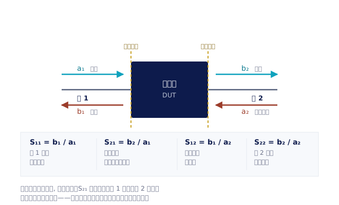
The S-parameter matrix of a two-port network can be written as two equations: b1 = S11·a1 + S12·a2 and b2 = S21·a1 + S22·a2. The notation is simple — Smn means 'the signal goes in at port n and comes out at port m', so the first subscript is the exit and the second is the entrance. Plenty of beginners get the order backwards, and end up confusing insertion loss with isolation.
S11 is the reflection coefficient at the input port: how much goes in, and how much comes back. In engineering it is usually expressed as return loss = −20·log10|S11| dB. A return loss of 20 dB means only 1% of the power is reflected, and it is a common acceptance threshold at the input of an antenna or a filter. Watch out for the difference in convention: a specification reading 'return loss ≥ 15 dB' is a positive number, but the S11 trace on the instrument screen is at −15 dB — they are the same thing.
S21 is the forward transmission coefficient. For a passive component (a filter, a cable, a connector) it converts into insertion loss = −20·log10|S21| dB; for an active component (an amplifier) the same S21 is the gain. A cable with 3 dB of insertion loss means half the power disappears inside it.
S12 is the reverse transmission coefficient — how much leaks back from the output to the input. For amplifiers, isolators and switches, this term is the isolation, or reverse isolation. Poor S12 means changes in the load feed back and affect the match at the input, which creates problems in system design. A reciprocal passive component satisfies S21 = S12, so if you measure the two as clearly different it is usually not that the component is remarkable but that the calibration or the connections are wrong — a very handy sanity check.
S22 is the reflection coefficient at the output port, symmetrical in meaning to S11. Obtaining all four parameters requires the signal to be launched from both directions; a four-receiver architecture (a reference and a measurement receiver at each test port) lets a VNA complete a bidirectional measurement without switching an internal changeover, and that is the hardware precondition on which the more advanced calibration methods depend.
S-parameters extend naturally to N ports: an N-port component has N² S-parameters, so a four-port component has 16. Balanced components are additionally described with mixed-mode S-parameters, which recombine four single-ended ports into differential and common modes and read out differential insertion loss, common-mode rejection and mode conversion directly. The R&S®ZNB has mixed-mode S-parameters built in and can measure balanced devices directly; the R&S®ZNBT uses a 'one reflectometer per test port' architecture in which up to 24 ports are all phase-coherent, with no external switch matrix required.
VSWR, return loss and reflection coefficient: three ways of saying the same thing
The most common confusion on the bench is treating voltage standing wave ratio (VSWR), return loss and reflection coefficient as three separate specifications. They are in fact three representations of the same quantity, and they convert into one another.
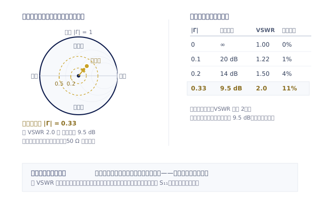
The reflection coefficient Γ is S11 itself, a complex number. Take its magnitude |Γ| and return loss (dB) = −20·log10|Γ|, while VSWR = (1 + |Γ|) / (1 − |Γ|). Going the other way, |Γ| = (VSWR − 1) / (VSWR + 1). The fraction of power reflected is |Γ|².
A few reference points worth remembering: |Γ| = 0.1 corresponds to 20 dB return loss, VSWR 1.22 and 1% reflected power; |Γ| = 0.2 corresponds to about 14 dB return loss, VSWR 1.5 and 4% reflected power; |Γ| = 0.333 corresponds to about 9.5 dB return loss, VSWR 2.0 and about 11% reflected power. The 'VSWR under 2' that antenna engineering so often quotes converts to a return loss greater than about 9.5 dB — by the standards of RF components, really rather loose.
Why keep three forms at all? VSWR comes from the ratio of the antinode to node voltage of a standing wave on a transmission line and is intuitive out in the field with antennas and feeders; return loss is expressed in dB and is convenient to add up with other dB quantities in a power budget; and the reflection coefficient retains phase, which makes it the only form usable for impedance transformation and matching design.
That also brings out an important limitation: VSWR and return loss retain magnitude only and have discarded the phase. They can tell you how good the match is, but not which way to go to fix it. To know whether the device under test is inductive or capacitive, and how much series inductance or shunt capacitance to add, you have to look at the complex S11 — that is, at the Smith chart. Every R&S VNA can display the same data simultaneously as log magnitude, VSWR, Smith chart and other formats; what you switch is the display format, and the measurement data underneath is one and the same.
Calibration is the crux: the instrument is not measuring only the device under test
This is the section beginners most need to take in. Power up a VNA, connect the device under test, and a trace appears on the screen — but that trace is not the S-parameters of the device under test. It is the sum of the analyzer's internal circuitry, the test cables, the adapters, the fixture and the device under test. The directional couplers inside a VNA have finite directivity and leak part of the incident signal into the reflected channel; the test ports themselves are not perfect 50 Ω (source match, load match); and the frequency response of the paths and receivers is not flat (tracking error). These are all repeatable, modellable systematic errors, and calibration is the procedure that measures them and then subtracts them mathematically from the result.
The error models have standard forms: a one-port reflection measurement requires three error terms to be corrected (directivity, source match, reflection tracking), while a full two-port measurement uses the widely adopted twelve-term error model, six terms in each direction. Solving for those unknowns requires measuring a set of calibration standards whose characteristics are already known — which is where the names of the various calibration methods come from.
SOLT (Short-Open-Load-Thru) is the most widespread method, and R&S's terminology calls it TOSM (Through-Open-Short-Match). It uses four standards — short, open, matched load and through — and its advantages are speed, directness and broad frequency coverage. Its premise is that the characteristics of those standards are accurately described: the fringing capacitance at an open end is normally modelled with polynomial coefficients, a short end has residual inductance, and every standard also has an offset delay. Those coefficients live in the calibration kit's data file, so the quality of the kit and the correctness of its data set the ceiling on the calibration. Use vendor A's coefficients to calibrate vendor B's standards and the result will be wrong, silently.
UOSM (Unknown Thru-Open-Short-Match) deals with a different reality: when the two test ports have connectors of different gender or different interface type (one N male, one 3.5 mm female, say), an ideal through cannot be made. UOSM allows the through section to be an unknown but reciprocal component, which the algorithm solves for. This requires a four-receiver architecture to work — the R&S®ZNH handheld vector network analyzer supports UOSM on exactly such a four-receiver architecture, so field work does not have to stack up adapters just to make the connectors meet.
TRL/LRL (Thru-Reflect-Line / Line-Reflect-Line) takes an entirely different route: it uses a length of transmission line itself as the primary standard, requiring only the line's characteristic impedance and length to be known, without having to model an open and a short accurately. On wafer, on printed circuit board fixtures, and in waveguide — anywhere standards cannot be plugged in and out — TRL is the most accurate. The price is limited bandwidth: a single line is valid only over the range where its electrical length gives roughly 20° to 160° of phase difference relative to the through, so covering a wide band usually means preparing several lines of different lengths. The R&S®ZNBT supports TOSM, TSM, TRL/LRL and UOSM as standard.
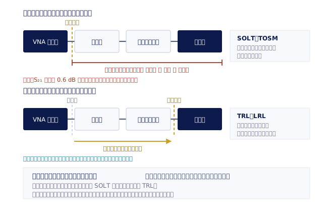
The most important idea once calibration is done is the reference plane: wherever the calibration standards were connected, the instrument now treats that position as a zero-length, ideal 50 Ω origin. Everything in front of the reference plane is subtracted, and everything behind it is counted as part of the device under test. So ideally the calibration is performed as close to the pins of the device as possible. When that is not achievable there are two tools: port extension shifts the reference plane by an electrical length and corrects only phase and delay, not loss or mismatch, which suits fine adjustment; de-embedding removes the fixture entirely using its own full S-parameter file, handling loss and mismatch together, and is the proper answer for fixtured measurement.
Two more habits are worth forming in practice. The first is to make good use of automatic calibration units: models such as the R&S®ZNLE support both manual calibration kits (R&S®ZN-Z1xx) and automatic calibration units (R&S®ZN-ZE1xx), which complete the procedure in a single connection and greatly reduce both the number of mating cycles and human error, while the guided calibration wizard on the instrument walks you through step by step. The second is always to verify after calibrating: measure one of the calibration standards again as though it were a device under test — a matched load should sit close to the noise floor, and a through should come out near 0 dB with flat phase. That one step catches nine out of ten failed calibrations in half a minute.
Nor is a calibration valid forever: temperature drift and connector wear will both invalidate it. Long-term stability is therefore a real cost item on a production line: the R&S®ZNB3000 has a phase temperature stability of 0.15°/°C, and the design goal is precisely to let a production line run continuously for days without frequent recalibration.
The four pitfalls newcomers hit most often
The first is connector torque and repeatability. At high frequencies the largest source of measurement uncertainty is often not the instrument but the connector. Precision coaxial connectors of the 3.5 mm, 2.92 mm, 2.4 mm and 1.85 mm families must all be tightened to their specified value with a torque wrench, and N-type connectors have a torque specification too; tighten by hand or over-tighten, and the result differs every time you connect — while the validity of a calibration rests on the assumption that the connection is repeatable. You should also check the centre conductor depth periodically with a pin gauge and keep connectors clean: one adapter with a pushed-in centre conductor can destroy an entire calibration kit. Once the calibration is done, try not to move the test cables either — the phase change caused by bending a cable is considerable at millimetre-wave frequencies, which is exactly why phase-stable test cables exist.
The second is port power and compression. When measuring a passive component, raising the source power improves the signal-to-noise ratio; but when measuring an amplifier, the source power has to be reduced until the device under test really is operating in its small-signal region, or the S21 you measure is already the compressed gain and not the small-signal S-parameter. At the same time, the amplifier's output power may exceed the safe range of the VNA's receiver, so an attenuator at the output or the receiver step attenuator must be used. The R&S®ZNH and R&S®ZNL both offer a receiver step attenuator option; the R&S®ZNA's output power covers −80 dBm to +17 dBm (ZNA26, under 10 MHz–4 GHz conditions) and reaches as low as −120 dBm with the optional step attenuator fitted, which is enough for small-signal measurements on high-gain components. A practical check: run a power sweep and see at which input power S21 starts to fall, and you will know whether your measurement point is still in the linear region.
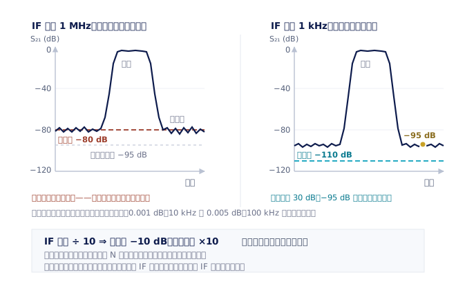
The third is the trade-off between IF bandwidth (IFBW) and sweep speed. A VNA's receivers down-convert the signal and capture it through an IF filter; the narrower the IF bandwidth, the lower the noise floor, the smaller the trace noise and the better the dynamic range — at the cost of a longer acquisition time per point. The rough rule is that reducing the IF bandwidth by a factor of ten improves the noise floor by about 10 dB and increases the sweep time by about a factor of ten (see Fig. 3). Which is also why any trace noise specification is meaningless unless read together with the measurement bandwidth — the R&S®ZNLE's typical trace noise of 0.001 dB is quoted at 10 kHz measurement bandwidth while the R&S®ZNA's 0.005 dB RMS is quoted at 100 kHz measurement bandwidth, and the two numbers cannot be compared directly. The practical answer is a segmented sweep: dense points and a small IF bandwidth through the filter passband to buy resolution and low noise, and a large IF bandwidth to run quickly through the out-of-band rejection region. Note in passing that too few points when measuring a narrowband filter will simply miss ripple and spikes, a common cause of wrong pass/fail decisions in production.
The fourth is fixtures and de-embedding. A surface-mount component cannot be plugged into a coaxial connector and needs a printed circuit board fixture, whose traces, vias and solder joints all get counted into the measurement. The available treatments, in increasing order of accuracy, are: port extension (delay only), fixture compensation, de-embedding with the fixture's S-parameter file, and performing a TRL calibration on the fixture itself. The R&S®ZNLE provides de-embedding and fixture compensation, while the R&S®ZNBT offers advanced embedding/de-embedding options conforming to IEEE 370 — a standard written precisely so that the quality of a de-embedding result can be quantified and compared. Another useful tool is time-domain analysis with time gating: transform the S-parameters to the time domain and you can see whether a reflection is happening at the connector, along the trace or in the device under test, and gate out the reflections that do not belong to it. The R&S®ZNL and R&S®ZNLE both offer the time-domain analysis option (R&S®ZNL-K2), and the same technique is used for distance-to-fault (DTF) measurement on cables.
From entry level to flagship: mapping the R&S VNA line-up
The R&S vector network analyzer line-up covers everything from teaching laboratories to millimetre-wave research, and selection turns mainly on four things: frequency ceiling, port count, dynamic range and sweep speed.
For entry-level and teaching use, start with the R&S®ZNLE, a compact standalone two-port instrument that measures S11, S21, S12 and S22 in full, with a built-in operating system and a 10.1 inch touchscreen and no external computer required. When one instrument has to cover several kinds of work, the R&S®ZNL is a three-in-one design — vector network analyzer, spectrum analyzer and power meter — and can be optioned with a lithium battery pack as a portable field instrument. For field work proper, look at the R&S®ZNH handheld vector network analyzer: a four-receiver architecture supporting UOSM calibration, 100 dB typical dynamic range, an IP51 ruggedised case, glove-friendly operation, and remote control from PC, Android and iOS.
The mainstay for development and general production is the R&S®ZNB, with up to 140 dB of dynamic range (150 dB with options), a 401-point sweep in just 4 ms, and built-in mixed-mode S-parameters, segmented sweep and embedding/de-embedding. High-volume production lines can consider the R&S®ZNB3000: a 1,601-point sweep in 11.7 ms, dynamic range up to 150 dB at 24 GHz, and expansion to as many as 48 test ports through a switch matrix. Multi-port devices — multi-port filters, phased arrays, automotive connectivity — map to the R&S®ZNBT, with up to 24 fully integrated, phase-coherent test ports and a fastest sweep of 2.5 ms for 201 points.
At the top sits the flagship R&S®ZNA, covering 10 MHz to 67 GHz (110 GHz with the ZNA67EXT), with system dynamic range specified at greater than 129 dB and 147 dB typical with the B3 option, and up to four phase-coherent internal signal sources on the four-port models — suited to advanced applications such as mixer and frequency converter characterisation, noise figure measurement, pulsed measurement and active load pull.