
What pre-compliance testing is, and why it exists
Electromagnetic compatibility (EMC) certification is a gate every product has to pass before it goes on sale. The difficulty is that an accredited laboratory often has a lead time of several weeks, a test day is not cheap, and on the day you usually get one chance. If a sweep turns up a frequency over the limit line halfway through, what an engineer can do on site is extremely limited: stick on some copper tape, add a few ferrite cores, change a cable, and hope. What is usually needed is a change to the board — and that means the whole schedule starts again.
Pre-compliance testing exists to absorb that risk. The idea is simple: the physics, the detectors and the measurement bandwidths that compliance testing is built on are all public and can be reproduced in your own lab; what is genuinely hard to reproduce is the validated test site. So find out on your own bench which frequency will exceed the limit, by how much, and where it is coming from, fix it there, and book the compliance test once you are confident.
This has to be stated plainly, with no hedging: pre-compliance results are not compliance results. Your bench has not been through site validation, the measurement uncertainty has not been evaluated, the ambient noise is not controlled, and the calibration chain of the equipment may not meet the requirements either. Pre-compliance data cannot be used to apply for a certificate, cannot go into the technical file as evidence of conformity, and cannot replace a report issued by an accredited laboratory. Its value lies in exactly two places: debugging, which tells you where the problem is; and risk judgement, which tells you what your chances are if you book the test now. Treating pre-compliance as 'the cheap alternative to certification' is the most common and most expensive misunderstanding there is.
KanTek Technology is an authorized dealer for R&S (Rohde & Schwarz), supplying pre-compliance measurement equipment such as EMI test receivers and near-field probes, with advice on selection and application; we do not, however, operate an accredited EMC chamber, and formal compliance testing still has to be commissioned from an accredited laboratory.
Two paths out: conducted emission and radiated emission
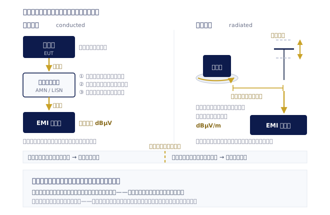
There are basically only two ways for the interference energy generated by the equipment under test (EUT) to leave the enclosure: along the wires, or radiated as an electromagnetic wave. The first is called conducted emission, the second radiated emission. Standards for most product categories regulate both, and they need completely different measurement set-ups.
The frequency at which the two divide is set by the applicable standard and is not necessarily the same for different product categories (domestic appliances, information technology equipment, automotive components, military equipment), so do not memorise numbers — understand the mechanism. At lower frequencies the product's power and signal cables are still short compared with the wavelength and are not efficient antennas, so the interference leaves mainly as current flowing along the wires and out onto the mains to bother other people — which is why what you measure is how much RF current or voltage there is on the line. At higher frequencies those cables, and the traces on the PCB, start to approach an appreciable fraction of a wavelength and become quite efficient antennas, so the energy simply leaves as an electromagnetic wave — which is why you switch to measuring field strength with an antenna at a set distance. The same noise source picks a different escape route at different frequencies; that is the only reason there are two measurement methods.
The key accessory for a conducted measurement is the artificial mains network (AMN), commonly known as a LISN (line impedance stabilization network). It does three things at once, and all three are indispensable. First, it presents the EUT with a known, stable RF impedance defined by the standard — without it, what you measure changes with which socket you plugged into today and what else happens to be connected to the laboratory mains, and is not repeatable at all. Second, it keeps interference carried on the mains itself outside, so that noise on the supply is not mistaken for emission from the EUT. Third, it provides a measurement port of known coupling so that the receiver can be connected without being exposed to the mains voltage. In other words, a conducted measurement without an artificial mains network produces floating numbers that cannot be compared with anything.
Another concept worth establishing is common mode versus differential mode. Differential-mode noise flows in opposite directions on the outgoing and returning conductors of the supply and is normally dealt with by X capacitors and differential-mode inductors; common-mode noise flows in the same direction on all conductors and returns through parasitic capacitance to ground, and is dealt with by Y capacitors and common-mode chokes. The overwhelming majority of radiated emission problems come from common-mode current, because that is the mechanism that turns a whole cable into an antenna. Fail to tell which one you are facing and the filter goes in the wrong place.
Why an EMI receiver is more than just a spectrum analyzer
The first question many engineers ask is: I already have a spectrum analyzer, so why do I need an EMI test receiver as well? Both display a spectrum, certainly, but an EMI receiver is built to an instrument specification such as CISPR 16-1-1, and the differences concentrate in three places: the detectors, the resolution bandwidth, and the front-end architecture.
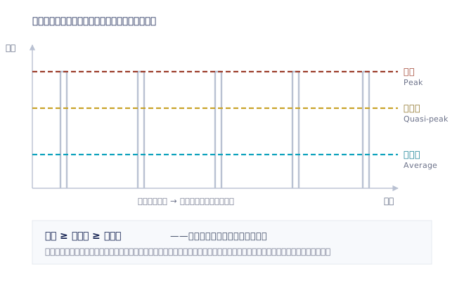
First, the detector. EMC measurements use at least three: peak, quasi-peak (QP) and average. Peak detection is the fastest and captures the largest value that occurred within the bandwidth, so its reading is always greater than or equal to the other two — which makes it ideal for sweeping quickly and picking out suspect frequencies. Average detection takes the mean of the envelope, suppressing impulsive noise and bringing out continuous carriers, which is good for telling a narrowband clock harmonic from sporadic switching noise.
Quasi-peak detection is the single most misunderstood thing in EMC measurement. It is not some kind of mathematical compromise, it is a deliberate model: what it models is how annoying the interference is subjectively to someone listening to the radio. It works by giving the detector a set of time constants that charge fast and discharge slowly — the signal appears and charges the detector rapidly, and once it goes the charge leaks away slowly. The result is that interference with a high repetition rate (nearly continuous) reads close to the peak value, while low-repetition sporadic pulses read much lower, because there is enough time between charges for the detector to discharge. That mirrors what the ear experiences: a continuous hiss is intolerable, a click once a minute is just about bearable. The time constants differ by frequency band and are prescribed by the applicable standard, and a quasi-peak measurement is very slow — which is the practical reason for sweeping fast on peak first and going back to run quasi-peak and average only at the few frequencies near the limit line.
Second, the resolution bandwidth (RBW). What an EMC standard prescribes is not 'whatever bandwidth looks nice' but a specific measurement bandwidth for each band, and CISPR bandwidths are defined at the −6 dB points whereas an ordinary spectrum analyzer conventionally quotes the −3 dB points. This means that even when two instruments show the same number on the front panel, their responses to a pulse will not be the same — and a large part of EMI noise is precisely impulsive. Which bandwidth to use in which band is governed at all times by the applicable standard; use the wrong bandwidth and the reading is meaningless and cannot be compared with the laboratory's result.
Third, the front-end architecture, the item most easily overlooked and most often responsible for false signals. The input to an EMI measurement is usually broadband, high-peak pulse energy, and the air is at the same time full of strong signals from broadcast stations and mobile networks. If the receiver front end is wide open, all that energy reaches the mixer together and pushes it out of its linear region, producing intermodulation products and spurious responses that do not exist on the EUT at all — and you spend an afternoon chasing noise the instrument made itself. An EMI test receiver puts a preselector ahead of the mixer: a bank of bandpass filters that track the tuned frequency, blocking energy outside the measurement frequency, followed by a low-noise preamplifier for sensitivity. The order matters — selectivity first, gain second. It is also why, on R&S EMI receivers, the preselector and preamplifier are usually listed explicitly as core or optional configuration items.
As for the models: the R&S®ESW is a high-end EMI test receiver reaching up to 44 GHz, compliant with CISPR 16-1-1 and MIL-STD-461; the R&S®ESR (9 kHz to 26.5 GHz) and R&S®ESRP (9 kHz to 7 GHz) carry the full set of detectors CISPR 16-1-1 requires — quasi-peak, CISPR average, RMS average and peak — with the ESRP additionally covering MIL-STD-461 and DO-160; and the R&S®EPL is a portable EMI test receiver covering 5 kHz to 7.125 GHz with CISPR quasi-peak, average and peak detectors built in, the closest of them to a bench instrument for pre-compliance work. Most models also offer a time domain scan option that uses an FFT to shorten a full sweep dramatically — which matters enormously when the debugging cycle is 'change one thing, measure again'.
Tracing the interference to its source on your own bench
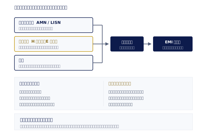
The full value of pre-compliance is not 'I measured 4 dB over the limit at 87 MHz', it is whether you can then work out within half a day which component or which length of trace is responsible. That takes two levels of measurement: a system-level sweep with an antenna or an artificial mains network, answering 'which frequency has a problem'; then a board-level search with a near-field probe, answering 'where is it coming from'.
There are two kinds of near-field probe. A magnetic field probe (H field, made as a small loop) is sensitive to current loops flowing in conductors and suits finding high-frequency current loops — the switching loop of a switch-mode supply, a long clock-driven trace, an inadequately decoupled power plane. An electric field probe (E field, made as a short stub) is sensitive to nodes with a high rate of voltage change — a switching node, an unbuffered high-speed clock pin, a heatsink. The practical technique is to park the receiver on the frequency you just measured over the limit (zero span or real-time spectrum mode), move the probe slowly across the board and watch where the reading jumps; having found a hot spot, turn the probe 90 degrees to confirm its directionality, then compare the two ends of the trace you suspect.
One thing has to be said first: a near-field probe gives relative values, not absolute ones. Its reading cannot be converted into a far-field field strength and cannot be used to decide whether a limit is met. Its only use is comparison — this point is higher than that one, this is lower after the change than before. Understand that and you will not waste time hunting for a calibration factor that does not exist. The R&S®HZ-15 EMC near-field probe set (30 MHz to 3 GHz) contains 2 passive E-field probes and 3 electrically shielded passive H-field probes, and can be used with the R&S®HZ-16 preamplifier (100 kHz to 3 GHz, 20 dB gain) to make weak signals easier to distinguish; if only magnetic field measurements are needed, the R&S®HZ-17 provides 2 H-field probes.
Having found the source, fix it at the source, not downstream. What that means is: deal first with the PCB layout (shrink the loop area of high-frequency currents, give every high-speed signal a continuous return path immediately adjacent to it, avoid crossing splits in a reference plane); then decoupling (where the capacitor sits and the inductance of its trace to ground usually matter more than its value); then the cables (common-mode chokes, how the connector end is grounded, whether the shield is bonded through 360 degrees); and only last the enclosure shielding (where success or failure depends almost entirely on apertures and seams, not on the thickness of the material). The reverse order — a filter at the output, a ferrite on every cable, conductive tape inside the enclosure — does often push the numbers down, but at the cost of bill of materials, assembly time and long-term reliability, and it is extremely fragile: change to a different batch of ferrites or move the harness once and the problem can come back.
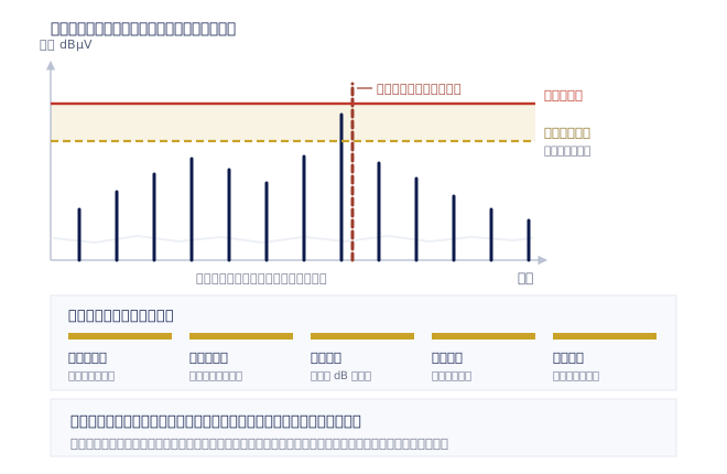
There is one more perspective that is regularly overlooked: look first at what the noise looks like on the spectrum. Evenly spaced 'comb' harmonics almost always come from a clock or a switching frequency — measure the spacing and you know the fundamental, and can go straight to the oscillator on the schematic; a broad, low hump is usually broadband noise from switching edges or the reverse recovery of a rectifier diode. Working back to the source from the shape of the spectrum is often faster than feeling around with a probe.
What separates your bench from an accredited chamber
Whether pre-compliance works for you depends on how clearly you understand the differences between your environment and the compliance test site. There are five main ones, and every one of them can shift the numbers by several dB.
First, the reference ground plane. The conducted test set-up at a compliance site fixes the relative positions of the EUT, the artificial mains network and the ground plane, because the parasitic capacitance from the EUT to ground directly determines the common-mode current loop. If your bench has no grounded copper surface, or the EUT sits at the front of the bench today and the back tomorrow, the common-mode content you measure moves with it.
Second, the measurement distance and the scanning routine. The distance for a radiated measurement is prescribed by the standard, and the test is not 'set the antenna up and measure once' — the EUT is rotated on a turntable, the antenna is raised and lowered through a range of heights, and horizontal and vertical polarization are both measured, all in order to find the maximum at each frequency. What you measure on the bench with one antenna at one fixed angle is almost certainly lower than the maximum the laboratory finds.
Third, cable placement. The size of this effect is unsettling. Cables are the main radiators, and their routing, their length, whether they are coiled and how far they sit above the ground plane all change the radiating efficiency. On the same EUT, simply rearranging the harness gives differences of several dB at particular frequencies as a matter of routine. So photograph and record the configuration when you do pre-compliance work, and rebuild the same arrangement for every measurement — otherwise you will not be able to tell whether the numbers improved because you changed the circuit correctly or because a cable ended up in a different place.
Fourth, the ambient. A compliance chamber exists in order to keep external signals out; your bench has broadcast stations, mobile base stations, office Wi-Fi, the LED lighting next door and an inverter air conditioner. That causes two kinds of error: mistaking an external signal for emission from your own product (and losing days chasing a problem that does not exist), or having your own emission hidden under something stronger in the ambient. The way to tell is simple and has to become a habit: switch the EUT off and sweep again with exactly the same settings. Overlay the two traces; only what appears when the EUT is powered is yours.
Fifth, the operating state of the EUT itself. Standards normally require measurement in the worst-case operating mode, not on a standby screen. Computing at full speed, every interface transmitting at once, motors at full load, the display showing a high-contrast pattern — emissions under those conditions can be a great deal higher than at idle.
Add those five together and you have the reason margin is essential. 'Just under the limit' on the bench amounts in substance to 'whether it passes certification is down to luck'. The practical approach is to set yourself an internal threshold stricter than the standard's limit, absorbing the uncertainty of the pre-compliance environment, the five configuration differences above, and the variation between production batches. There is no standard answer for how much margin to leave; it depends on how close your measurement environment is to the compliance configuration and how much your product varies. But making 'there is margin' the release condition is far safer than making 'it did not exceed the limit' the release condition.
A practical pre-compliance route
Collapsing the preceding sections into an order you can actually work through, it goes roughly like this: confirm which standard and which product category apply to your product (get this step wrong and everything after it is wasted, so ask the accredited laboratory if you need to); build the conducted measurement set-up, the important parts being the artificial mains network and a grounding and placement arrangement that stays fixed; sweep the whole band on peak detection and pick out the frequencies near the threshold; run quasi-peak and average measurements only at those frequencies; use near-field probes to trace every over-limit frequency to a specific place on the board; make changes in the order layout, decoupling, cables; remeasure in exactly the same configuration after every revision and keep the data; and only when there is enough margin against your own internal threshold, book the accredited laboratory.
There is no single right answer on equipment, which depends on the upper frequency you need to cover and where the work is done. For day-to-day debugging at an R&D bench, mainly conducted and lower-frequency radiated measurements on domestic appliances or IT products, a portable EMI test receiver of the R&S®EPL class (5 kHz to 7.125 GHz) with a near-field probe set will usually cover the overwhelming majority of debugging needs; where commercial, aerospace (DO-160) and military (MIL-STD-461) configurations all have to be supported, the R&S®ESRP (9 kHz to 7 GHz) and R&S®ESR (9 kHz to 26.5 GHz) offer a more complete set of compliant detectors and bandwidths; and where measurements extend into the millimetre-wave bands, or the highest performance is needed for an in-house test site, that is the territory of the R&S®ESW (up to 44 GHz). If a radiated measurement lacks sensitivity because of the distance between the antenna and the EUT, an EMI/EMC preamplifier and signal conditioning unit such as the R&S®ESCU (0.1 GHz to 18 GHz) can improve the system noise floor.
Finally, back to the mindset. Pre-compliance is not there to replace the accredited laboratory, it is there so that the day you walk into one holds no surprises. It moves the moment of discovery out of a setting that takes weeks to book, costs a good deal and leaves no room for unhurried debugging, and back onto your own bench — where you can solder in a capacitor, revise a layout and measure again immediately. The speed of that cycle is what pre-compliance is really buying.