
Why RF measures power rather than voltage
Measuring voltage is the most natural action in a low-frequency circuit: put the probe on the node and the value you read is that node's voltage. At radio frequency, though, the wavelength of the signal is of the same order as the length of the circuit, and voltage amplitude varies with position along the transmission line. Wherever a standing wave exists, the voltage you measure at different points on a coaxial line is a different number — the reading depends on where you put the probe rather than on how much energy the system delivered.
Power is different. On a lossless transmission line the power travelling to the load is conserved along the line; whichever section you measure at, the figure means the same thing. That independence from position is the first reason RF measurement takes power as its base quantity.
The second reason is more practical: power is what the system cares about anyway. Transmitter output, receiver sensitivity threshold, amplifier compression point and saturated output, regulatory emission limits, a component's damage threshold — all of them are defined in power. As for the familiar P = V² / R, it holds only if the impedance is known and the waveform is known, and on a real RF chain neither premise usually holds.
One more point: an RF probe brings its own impedance into the circuit, so the act of measuring changes the thing being measured. A power sensor takes another route — it is a very well-made 50 Ω load that absorbs the power and measures it. Every definition in power measurement is therefore built on a reference plane: how much power was absorbed at the plane of the sensor's connector. That idea comes back later when we discuss attenuators and couplers.
dBm, dBW and watts: dB is a ratio, not an absolute value
The absolute unit of power is the watt (W). But RF power spans too wide a range — a receiver noise floor may be of the order of 10⁻¹⁵ W while a transmitter is measured in kilowatts — and linear units are awkward to write and awkward to compute in your head, so the industry works in logarithms.
dBm is logarithmic power referred to 1 mW: dBm = 10 × log₁₀(P / 1 mW). So 0 dBm is 1 mW, +30 dBm = 1 W, −30 dBm = 1 μW. dBW is referred to 1 W, so 0 dBW = +30 dBm, and the two always differ by 30.
The commonest mistake — and the one most often found in reports — is this: dB is not a unit of power. dB expresses a ratio of two powers, and gain, attenuation, dynamic range, noise figure and peak-to-average ratio are all in dB. dBm is absolute power. The arithmetic therefore runs: dBm + dB = dBm (a signal passing through gain or attenuation); dBm − dBm = dB (two powers compared); and dBm + dBm has no physical meaning. Saying 'the attenuator brought the signal down to −20 dB' is wrong; the correct statement is 'attenuated by 20 dB' or 'down to −20 dBm'.
A few mental benchmarks are worth having: +3 dB is about twice the power, +10 dB is ten times, −3 dB is half. So +23 dBm is about 200 mW and +43 dBm about 20 W. For judging on the spot whether a reading is plausible, this is faster than reaching for a calculator.
Three families of sensor, and what each suits
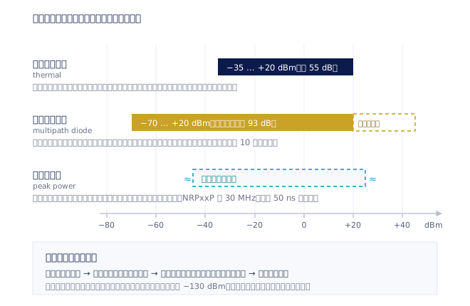
The thermal / thermocouple sensor works in the most direct way: convert the RF power to heat and measure the DC voltage a thermocouple produces from the temperature difference. Because it measures the energy itself, it is entirely indifferent to waveform — CW, pulsed or any complex modulation, what it reads is the true average power. Its linearity is excellent and it can be traced directly to a DC power standard, which is why it is often used as a calibration reference. The price is speed (the thermal time constant limits how fast it responds) and a lower limit set by thermal noise, giving a narrower dynamic range than a diode. The R&S®NRPxxT series belongs to this family, covering DC to 170 GHz (coaxial and waveguide models together) with a measurement range of −35 dBm to +20 dBm; that roughly 55 dB range is the characteristic thermal-sensor trade-off.
The diode detection sensor rectifies with a Schottky diode. At very low power the diode works in the square-law region, where the output DC voltage is proportional to input power — and there it too measures true average power, independently of waveform. But once the power rises and leaves the square-law region, the diode starts responding to the envelope peak instead and the reading begins to vary with waveform. This is the one thing a user of diode sensors most needs to understand: its 'linear region' is not about the reading being linear, but about whether it still faithfully reflects average power.
The modern answer is a multipath architecture: the signal is distributed to several diode paths with different amounts of attenuation so that each stays inside its own square-law region, and the sensor combines them internally. Three-path diode sensors such as the R&S®NRPxxS / NRPxxSN can therefore offer up to 93 dB of dynamic range in a single sensor (about −70 dBm at the bottom for the standard model, up to +45 dBm at the top for a high-power model — these are different models, not one continuous range on one sensor), give the correct average power for modulated signals such as GSM, LTE/LTE-A and 5G NR, and reach measurement speeds of up to 100,000 readings per second. Where requirements are simple and the budget is limited, the entry-level R&S®NRPxE is a plain diode USB sensor with 80 dB of dynamic range (−60 dBm to +20 dBm) and 100 kHz of video bandwidth, still supporting trace and time-gating modes.
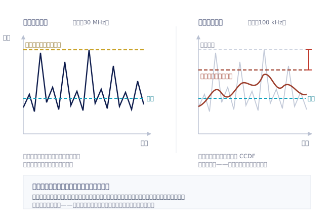
The peak / wideband sensor has an entirely different goal: to record how power changes with time. The critical specification here is video bandwidth, which decides how fast an envelope change the sensor can follow; where video bandwidth is insufficient, the peak measured is smoothed away and reads systematically low — the commonest source of false data in pulse measurement. The R&S®NRPxxP wideband peak and pulse power sensors have up to 30 MHz of video bandwidth, an 80 Msample/s sampling rate (12.5 ns time resolution) and can measure pulses as short as 50 ns, which is exactly what radar pulses and wideband modulation call for.
There is also a frequency-selective approach. The R&S®NRQ6 down-converts and filters inside the sensor and measures only the power in a channel you specify (measurement bandwidth up to 100 MHz), so its lower limit reaches −130 dBm — suitable for measuring a single signal in an environment with interference, spurious signals or several coexisting carriers, which a wideband terminating sensor cannot do, because a wideband sensor sums up everything in the band.
The selection principle condenses into three sentences: for an absolutely correct, traceable average, use thermal; for wide dynamic range plus speed, use a multipath diode; to see the envelope and measure pulse parameters, use a peak sensor. A real project often needs more than one of them.
Why average power lies about a modulated signal
For a pure CW carrier, the average power is the whole story. But as soon as a signal is modulated, or chopped into pulses, average power is only a figure diluted by time; it no longer tells you how strong the signal is at any given instant.
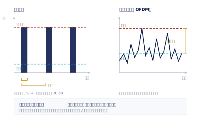
The quantity that describes the gap is crest factor, usually expressed in the power domain as PAPR (peak-to-average power ratio) in dB. CW has a PAPR of 0 dB. The rectangular pulse is the most intuitive case: average power = peak power × duty cycle. So a radar pulse at 1% duty cycle has an average power 20 dB below its peak — the power meter displays +10 dBm while what is actually hitting the device under test is +30 dBm. That gap is enough to destroy a sensor or an amplifier stage.
Digitally modulated signals are more awkward still, because they have no fixed duty cycle. For a multicarrier signal of the OFDM type the instantaneous envelope is the outcome of a statistical distribution, with PAPR commonly around the 10 dB level and varying with resource allocation and waveform configuration. Whether an amplifier enters compression, and whether the distortion figures exceed their limits, depends on those occasional peaks, not on the average.
The old way of dealing with this was 'duty cycle correction': enter the duty cycle into the power meter and let it convert from average power back to pulse power. That only works if the pulse is an ideal rectangle and the duty cycle is precisely known; for shaped pulses with rise and fall edges, or for a real modulated signal, it gives a wrong answer.
The correct approach is time gating: use a peak sensor with sufficient video bandwidth to capture the power-versus-time trace, then define one or more gates and average only inside them. That is what gives the true burst power, and it also yields peak power, rise and fall times, pulse width, repetition frequency and duty cycle in the same measurement.
A way to remember it: average power answers 'how big a thermal load is this', and peak power answers 'will it compress, will it burn out'. With a modulated or pulsed signal, both questions have to be answered.
Where the accuracy actually goes: mismatch, calibration factor and zeroing
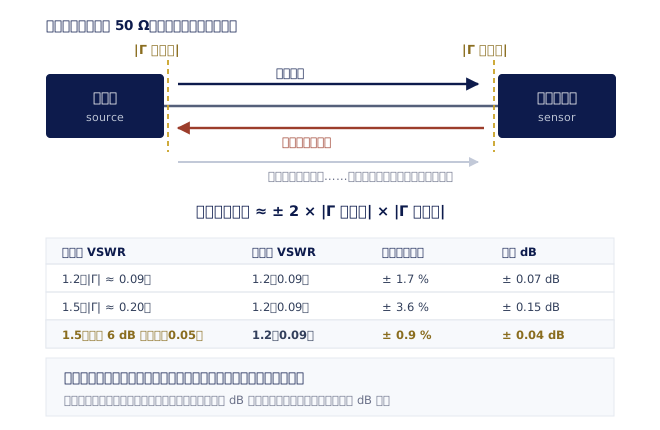
Mismatch uncertainty is usually the largest single item in a power measurement's error budget, and it has almost nothing to do with how expensive your power meter was. The reason: neither the source's nor the sensor's impedance is an ideal 50 Ω, the reflection coefficients Γ at each end form a standing wave between them, and the power actually absorbed by the sensor floats within a range depending on the phase relationship between the two. You have no way of knowing that phase, so the whole range has to be carried as uncertainty. As a rough estimate, that range is about ±2 × |Γ_source| × |Γ_sensor|.
The number is larger than most people's intuition. Even with a VSWR of only 1.2 at both source and sensor (|Γ| about 0.09), mismatch contributes about ±1.7% of uncertainty (roughly ±0.07 dB), the same order as the sensor's own linearity error or larger. It gets worse with frequency, because VSWR generally degrades as frequency rises.
There are two ways to reduce mismatch uncertainty: choose sensors and adapters with good VSWR, or put a good-quality attenuator or isolator in front of the sensor, since an attenuator improves the mismatch the source 'sees' by about twice its attenuation in dB. The price is the loss of measurement range at the low end, so this is a decision to be taken project by project rather than something to do always.
The second source of error is the calibration factor. A sensor's effective efficiency varies with frequency, so the power meter has to know the carrier frequency before it can apply the right correction. Traditionally this meant reading a table on the sensor body and entering it by hand; a modern USB power sensor stores the whole calibration data set inside the sensor and applies it automatically once the frequency is set. But 'automatic' does not mean 'nothing to do' — measure at 28 GHz while the setting is still at a default of 1 GHz and the error can be of the order of a dB, with a reading that looks perfectly normal.
Third is zeroing and reference calibration. Zeroing removes the DC offset and drift of the sensor and measurement chain, and has to be done with the RF genuinely off — switching off the source's output key does not necessarily mean no RF is leaking, and the safest course is to disconnect, or to use the sensor's built-in zeroing function. The closer you work to the bottom of the measurement range, the more critical zeroing is, and it should be repeated after any significant change in ambient temperature. Traditional bench power meters also use a 50 MHz / 1 mW reference source on the front panel for gain calibration; modern USB sensors are calibrated individually at the factory and carry their own traceability, needing no external reference — but they still have to be returned for calibration on schedule, or that traceability is only nominal.
Once it is in the system: attenuators, directional couplers and the measurement plane
Back to the idea of the reference plane: put anything in front of the sensor and the measurement plane has moved, and it is up to you to account for it.
An attenuator is the commonest example. Its attenuation has to be entered into the power meter as an offset, or the reading is wrong by exactly that many dB. The attenuation also varies with frequency and has an uncertainty of its own, and both belong in the error budget. An attenuator is almost unavoidable when measuring a high-power transmitter (it also protects the sensor from destruction), but it raises the bottom of the measurable range by the same amount, which has to be worked out in advance when the signal has a large dynamic range.
A directional coupler takes a small fraction of the power off the main line and feeds it to the sensor, so the system can monitor power continuously while operating normally, with no need to break the chain. Two specifications matter in use: the coupling factor (again entered as an offset), and directivity. With insufficient directivity the reverse wave leaks into the forward port and the error in a reflected-power measurement becomes very large indeed — the trap most easily overlooked when measuring antenna return.
If the goal was 'what actually happens between the transmitter and the antenna' in the first place, then the right tool is a through-line directional power measurement: put the sensor in series with the chain, measure forward and reflected power at the same time, and obtain VSWR or return loss directly. The R&S®NRT2 directional power meter (power reflection meter) is designed for this, covering 25 MHz to 4 GHz, with average power measurement from 3 mW to 120 W and peak envelope power (PEP) up to 300 W (the actual ranges depend on which directional sensor is fitted). A terminating sensor cannot answer questions of this kind, because it has to absorb the power.
Finally, integration. When several channels have to be watched at once (forward and reflected, say, or each port of a multiport device), or when external triggering, limit monitoring and analogue voltage output — the sort of functions automated testing uses — are needed, that is the case for a base-unit power meter. The R&S®NRX comes standard with one measurement channel and expands to two or four, and works with the R&S®NRP series of USB power sensors, the NRQ6 and the NRT-Z directional sensors, so one mainframe covers average, peak and through-line measurement alike.